


Data is becoming an integral part of everyday life. Even if we are not fully aware of it, we deal with it all the time and it affects our lives in significant ways. This blog post elaborates on a particular type of data: time series. If you want to know more and discover what problems you can solve with time series analysis, you've come to the right place.
Machine learning in the network domain - introduction
Have you ever wondered how much data is created (including newly generated, captured, copied, or consumed data) each day? Currently it is 0.33 zettabytes ![]() every day! It is worth noting that one zettabyte is 1,000,000,000 terabytes. This is an almost unimaginable number. What's more, this value is steadily increasing. In the 13 years starting from 2010 we have seen a 60-fold increase in this number. It is estimated that in two years' time, i.e. in 2025, the amount of data created will be 50% higher than in 2023 and will reach a value of around 181 zettabytes. In addition, the way this data is transmitted is also changing. In Q1 2023, about 60% of website traffic
every day! It is worth noting that one zettabyte is 1,000,000,000 terabytes. This is an almost unimaginable number. What's more, this value is steadily increasing. In the 13 years starting from 2010 we have seen a 60-fold increase in this number. It is estimated that in two years' time, i.e. in 2025, the amount of data created will be 50% higher than in 2023 and will reach a value of around 181 zettabytes. In addition, the way this data is transmitted is also changing. In Q1 2023, about 60% of website traffic ![]() came from mobile devices, a big increase from Q1 2015 when it was about 30%.
came from mobile devices, a big increase from Q1 2015 when it was about 30%.
Moreover, new data sources are emerging. For example, it is predicted that the number of Internet of Things (IoT) devices in Q1 2023 will almost triple from 9.7 billion in 2020 ![]() to more than 29 billion in 2030. We can definitely and undeniably see an advancing wave of digitization - this is the information revolution, where the ability to transfer information securely, reliably, and rapidly is key. As you probably know, this is what networks are for. And network technology is under constant development to support this rapid progress.
to more than 29 billion in 2030. We can definitely and undeniably see an advancing wave of digitization - this is the information revolution, where the ability to transfer information securely, reliably, and rapidly is key. As you probably know, this is what networks are for. And network technology is under constant development to support this rapid progress.
There are many challenges in today’s networks. The network environment as such is highly heterogeneous. Each network domain is unique and it can differ in terms of technologies, mechanisms, protocols, etc. Another issue is the evolution over time of each network through, for example, the constant increase in the number of applications running on the network and the types of devices connected. Network operations and management, due to their complexity and continuous changes, remain cumbersome, and the faults that occur are very often due to human error.
Therefore, the idea of introducing mechanisms for self-configuration, self-fixing, self-optimization, and self-protection within networks has been around for some time. Such mechanisms seem to be justified as it is almost impossible to manually keep up with the administration of such a complex environment that changes over time. Approaches such as software-defined networking (SDN) and recently the application of machine learning techniques can help to address the general need for automation and intelligence in networks.
Machine learning is a technology domain, a collection of algorithms and methods that can learn from past experiences collected in the form of data. The main goal of these algorithms is to provide high-quality predictions for data that is not visible during the training process. The capabilities of these algorithms allow not only the extraction of human-visible knowledge, but also the discovery of hidden relationships contained in the data. Their high level of usefulness is also evidenced by their ability to make automatic decisions and process very large and extremely complex data sets that are impossible to analyze manually. Machine learning has demonstrated its great usefulness in tasks such as regression, classification, clustering, time series analysis, image, audio, video analysis, and analysis of data of many different types. From a network point of view, the most common types are graph data and time series data. Our focus in this blog post is on the latter. The basic problems considered for time series are defined and briefly discussed here. Practical examples of applications in a network context are also presented.

Definition of a time series
A time series is an ordered collection of measurements of a certain quantity. The order of measurements is selected individually depending on the nature of the problem under consideration. The most common is ordering according to the time of a single measurement, which usually takes place at equal intervals, such as once per second, minute, hour, or day, and so on. It is also possible, but not common, to encounter ordering according to another dimension, such as space. For example, we can take temperature measurements at different locations in the northern hemisphere located at the same longitude and order them by latitude.
Time series are definitely a type of data we encounter every day. In business and economics, we encounter daily closing stock prices, weekly interest rates, monthly price indexes, etc. In meteorology, we may meet hourly measured wind speeds, daily temperature, or atmospheric pressure measurements. In medicine, we can encounter EEG (electroencephalograph) and ECG (electrocardiogram) signals, which are also time series. Also, in the network context, time series are ubiquitous - you can measure various data over time, e.g. the traffic flow bit rate, packet rate, packet delays, packet jitter, requests rate, CPU/memory consumption, etc. Figure 1 shows an example traffic flow bit rate in different time scales (daily, weekly and monthly) with hourly measurements.
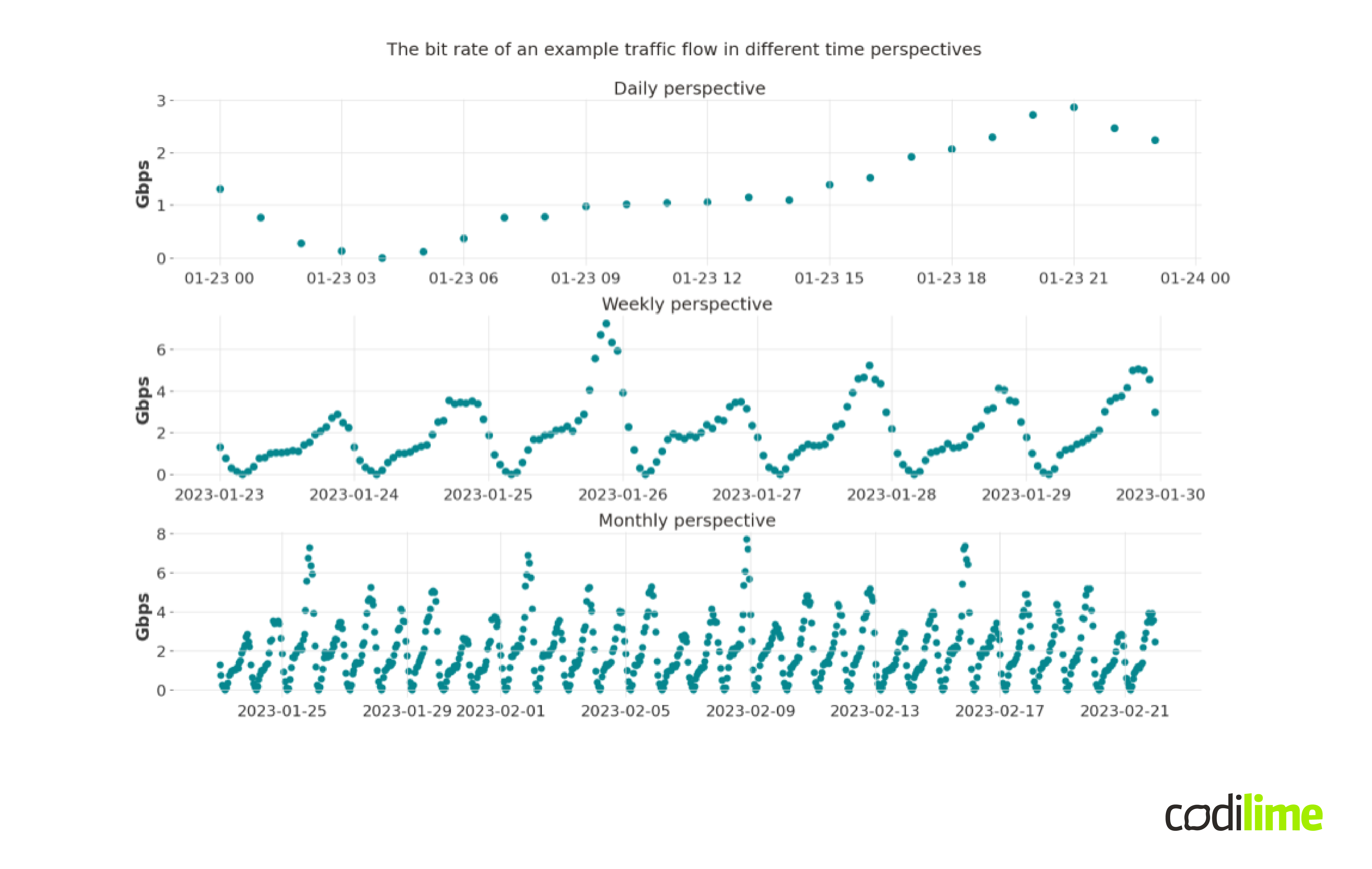
The measured rates for the first chart range from values close to zero to values around 3 Gbps. On a weekly basis, the values range from about 0 to about 6 Gbps, and on a monthly basis from about 0 to 8 Gbps. What is definitely striking is the strong, recurring, regular pattern. Apparently, there is some kind of link between the values in the different timestamps that ties it all together. Let's try to describe such a connection and start with the concept of a random variable.
A random variable describes a measurement of some quantity, the result of which is uncertain. Uncertainty can arise both from a deficiency in our knowledge of the phenomenon under consideration but also from its essentially random nature. A good example would be a throw of a dice. The result of the throw can be a number from 1 to 6. The throwing process itself is extremely complicated. The force with which the cube is thrown, to what height it is thrown, and at what speed rotates around its axis - all these elements matter for the final result of the throw. But factors such as the movement of the air in the room during the throw, the curvature of the floor on which the cube will fall, and many others also have an impact.
So, instead of trying to describe directly the complicated process of throwing a dice, (because it is impossible to take into account all the factors that affect the final result), you can use a probabilistic (random) description and the concept of a random variable. In this case, the random variable will be the result of a dice throw which is uncertain. Let's denote this result by X. The values that X can take is a natural number from 1 to 6. If the dice is fair, i.e. not loaded, then any result should, due to the symmetry of the dice, appear with a probability of 1/6. We denote the result of a single throw by X(ω), where ω denotes the state of the world at the time of the throw.
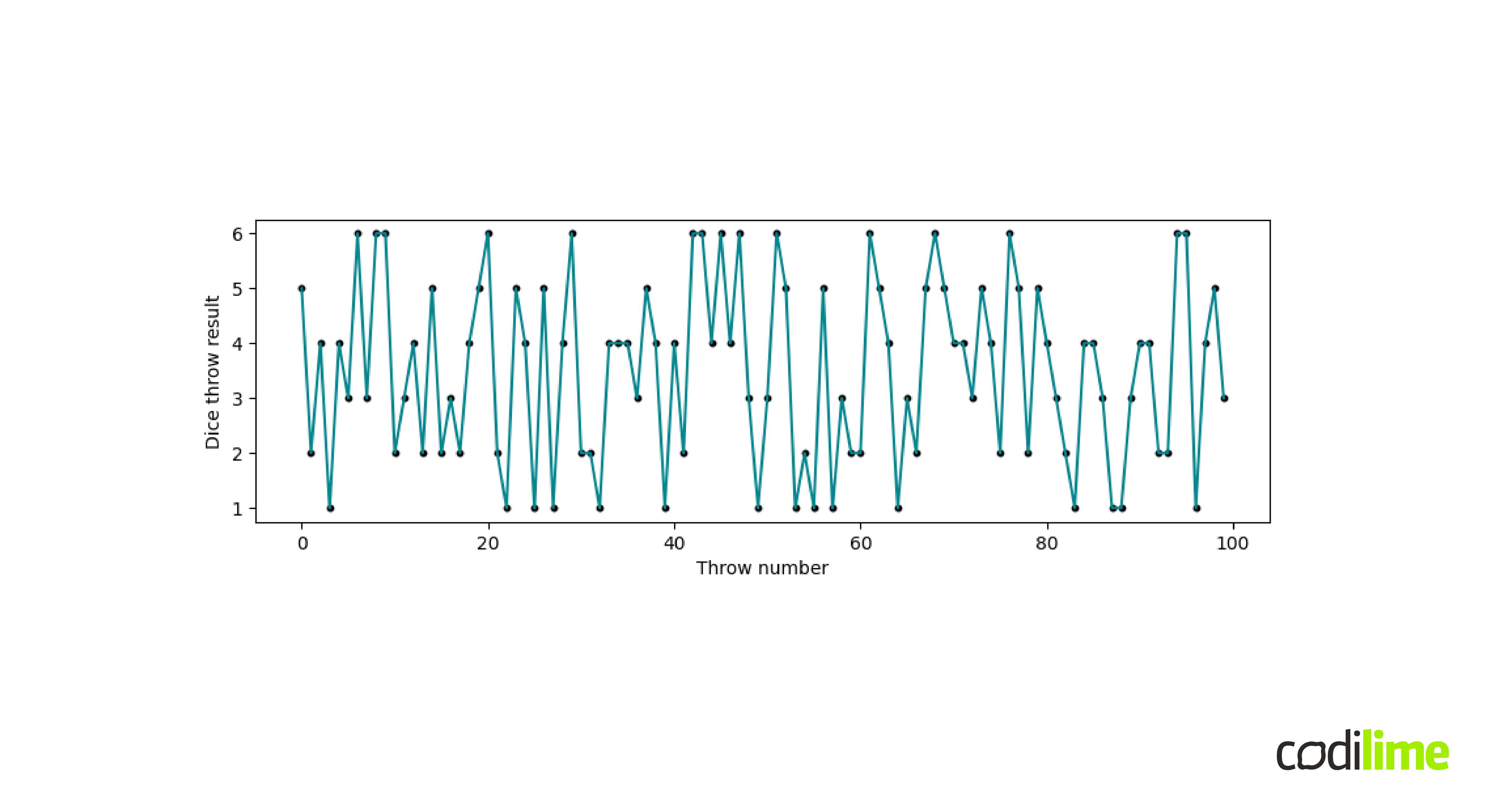
Of course, under normal conditions each successive throw is independent of the previous one. An example of such a series of independent dice throws is shown in Figure 2. There is no particular relationship between the consecutive results of the dice throws. Such a time series is called white noise and cannot be forecast accurately. White noise is often used in modeling and is a part of the signal not explained by our model.
Now, let's try to introduce a kind of dependence. Let's make a series of dice throws and keep adding together the results of the throws. If we cross, say the 60-point barrier, instead of adding the result of the throw, we start subtracting it until we finally reach the zero-point barrier, and then we start adding the results of the throws again. The process continues, and an exemplary result of 300 throws is shown in Figure 3.
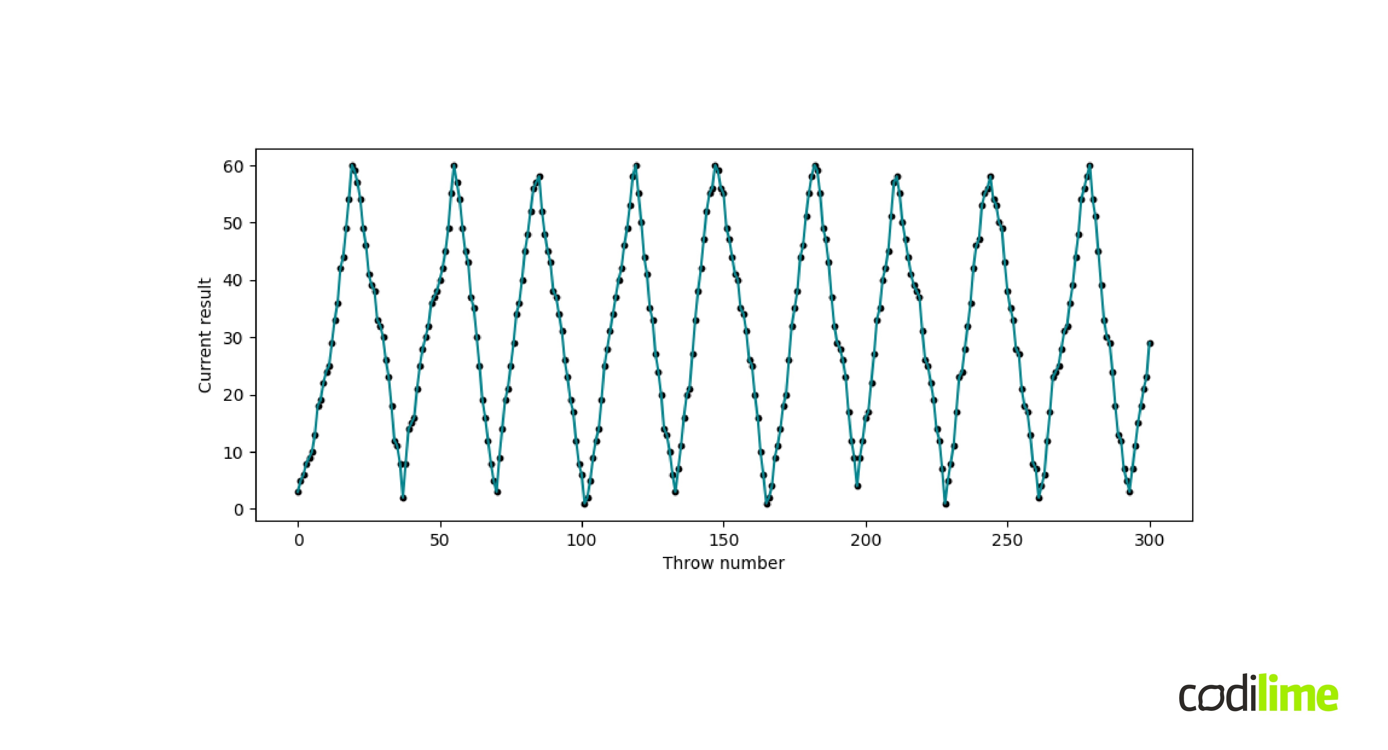
The relationship across time of the obtained results is clearly visible, it was introduced manually and is rather simple. In the case of Figure 1, the source of the time dependence between different points of the time series is hidden, but its effect is clearly observable. What's more, such a relationship in time is very important from the perspective of the problems and tasks we will define in the following sections, because it actually constitutes the essence and differentiates the individual time series.
In each timestamp, we can associate a random variable with the value of the time series. This illustrates our uncertainty about the value of the time series at a given time point. As in the example of throwing a dice, only as a result of the measurement did we get an ordered set of numbers. In the context of Figure 1, as a result of the measurement, we get the following collection of numbers:
Xt=2023-01-25 00:00:00 (ω), Xt=2023-01-25 01:00:00(ω), Xt=2023-01-25 02:00:00(ω), ... (1)
where Xt=2023-01-25 00:00:00, Xt=2023-01-25 01:00:00, Xt=2023-01-25 02:00:00, ... are the underlying random variables associated with the time series value at specific timestamps. Using mathematical nomenclature, the ordered sequence of random variables is called a stochastic process and its realization (1) is called a time series.
Time series forecasting
Time series forecasting is the task of forecasting the future values of a time series based on its historical values. In order to correctly define this problem, it is also necessary to decide on the size of the forecasting horizon h, i.e. how many observations into the future we want to forecast. Having already defined the problem, i.e. specified the time series we want to forecast with a certain time granularity and a specified forecasting horizon, we can get down to building the forecasting algorithm. For this purpose, we can reach for one of the existing approaches, many of which can be assigned to one of two categories: statistical models that rely on far-reaching assumptions about input data, and machine learning methods that make no such hard assumptions.
Time series forecasting is one of our data science services. Click to read more about them.
It is often the case that several methods and models are used to create the final forecasting algorithm. Statistical models can be described as those that assume the form of the stochastic process that generated the time series under consideration. That is, a connection is postulated linking present observations to past ones, and the observed series is assumed to be derived from such a process. A good example is the AR(p) ![]() model (autoregressive model), where p is a parameter, a natural number that must be specified prior to the training process. When p=1 the model takes its simplest form and is then as follows
model (autoregressive model), where p is a parameter, a natural number that must be specified prior to the training process. When p=1 the model takes its simplest form and is then as follows
Xt=α * Xt-1+∈t, (2)
where Xt, Xt-1 are the observations at timestamp t and the moment earlier t-1 and ∈t is a noise signal at timestamp t and α is a real number. The equation (2) reflects the linear relationship between past and current state at timestamp t. The goal is to find the value of the parameter α that best fits the observed historical values in a process called training which will not be further analyzed in this article. Another decision to be made is the number of historical observations that we want to use in the training process. This is also an important part in the process of building the forecasting algorithm. As an illustration, let's take the traffic shown in Figure 4.
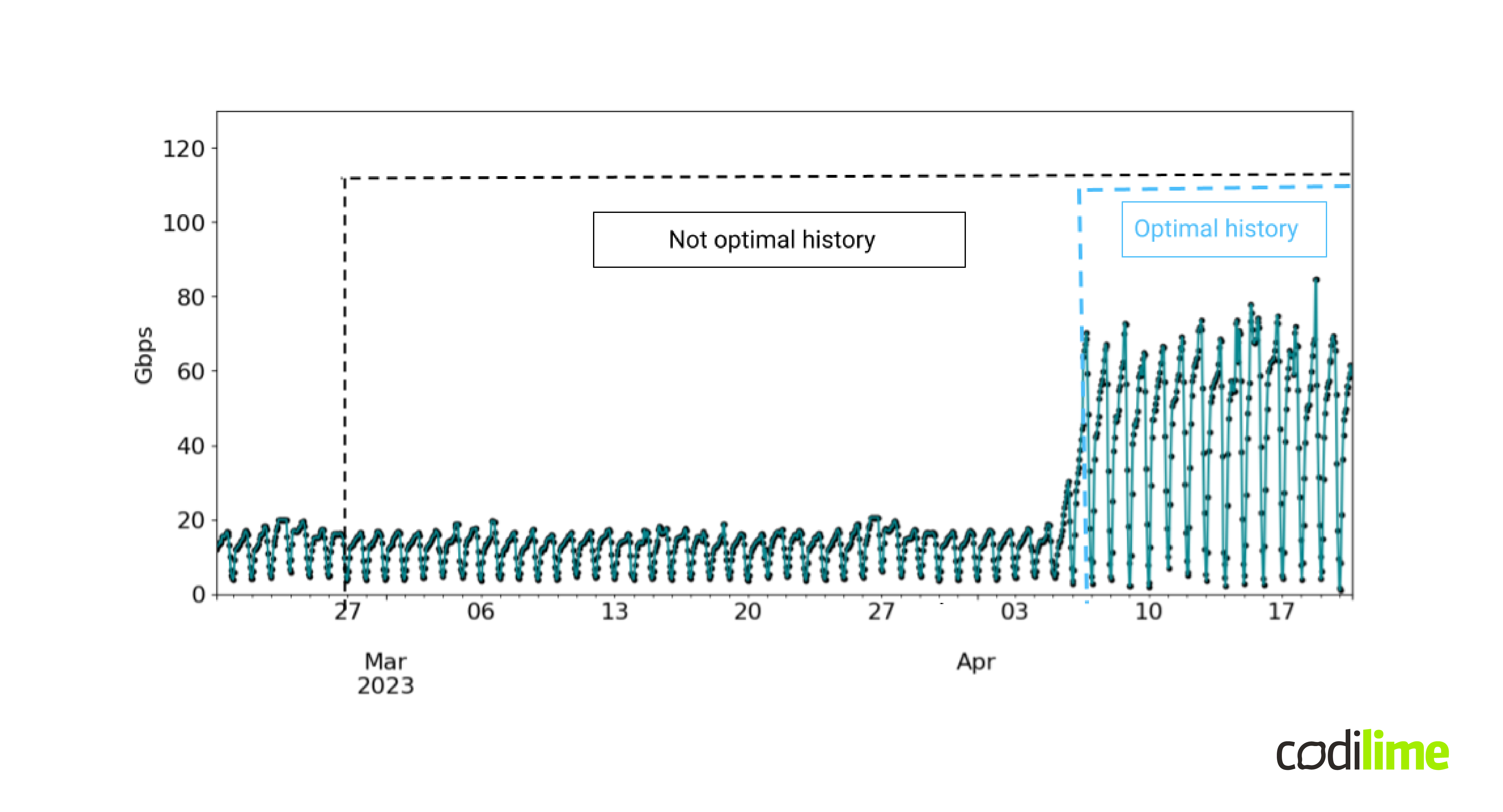
We can observe a step change in the traffic flow bit rate on April 7, 2023. (e.g. due to a routing change in the network, some network policy update, the addition of new clients to the network, or some other reason) Using the history contained in the black box in the training process, we mostly introduce traffic with characteristics that are not currently valid. This can result in low-quality forecasts due to the inertia of each model/method in keeping up with the latest changes occurring in the observed time series. Therefore, to get a better quality forecast, it may be more optimal to use a shorter history, the one included in the blue box. The size of the history used in the learning process is an example of a hyperparameter, i.e. a parameter whose value cannot be determined in the learning process itself (another example is the p parameter in the AR(p) model). In practice, this is done manually using intuition and professional experience, but there are also automatic methods using cross-validation and algorithms such as the tree-structured Parzen estimator algorithm or Gaussian process.
As already highlighted, the forecast horizon is of practical importance for building a forecasting algorithm. You mostly hear about short-term and long-term forecasts. At the same time, the boundary between these two terms is fluid and depends individually on the nature of the data under consideration and the business purpose you want to use the forecast for. Nevertheless, in the case of long-term forecasting, it often turns out to be very beneficial to use decomposition approaches, i.e. decomposition of the considered time series into components, which are modeled and forecasted separately and finally glued together into one final forecast. This is a manifestation of the divide-and-conquer paradigm in the context of time series. As an example of a decomposition approach that can work well for time series that show some seasonality (e.g. daily, weekly, quarterly, yearly), you can take the additive decomposition model into the trend, seasonality, and residual. The STL additive decomposition (Seasonal and Trend decomposition using Loess) for an example traffic flow is shown in Figure 5.
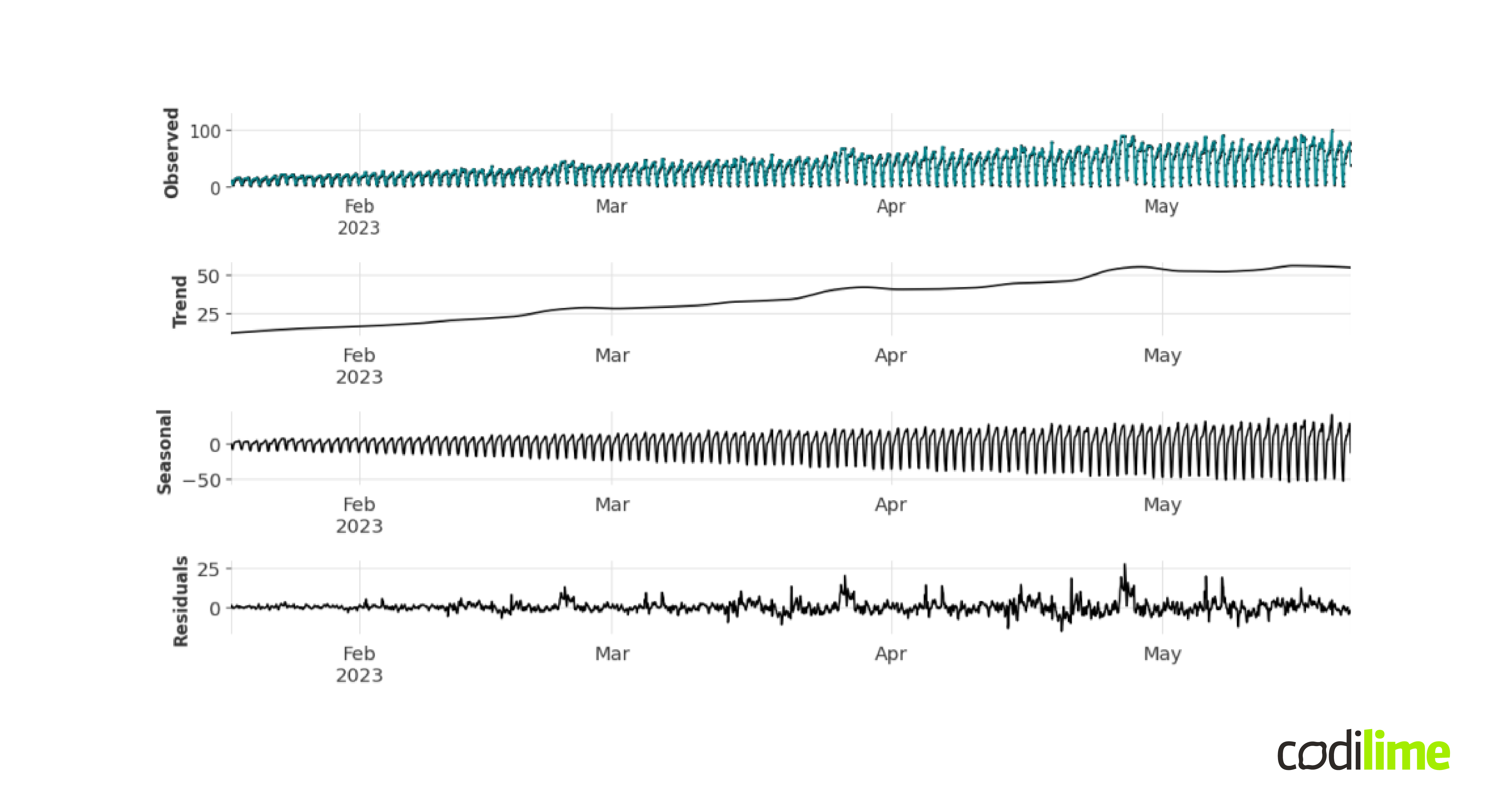
The trend component reflects the long-term progression of the time series, the seasonal component reflects the seasonal behavior, and the residual signal represents the remainder of the signal. The input time series is the sum of these three components, hence the name additive decomposition. From the perspective of long-term forecasting, the ability to forecast the trend plays a significant role. In the example presented in Figure 5, the trend took the rather simple form of a linear function, but in real-life use cases, it can take very complex forms. For short-term forecasts on the other hand we can model the trend component with a flat line, which is why long-term forecasting is usually considered more challenging. There also exist more sophisticated decomposition techniques, such as singular spectrum analysis (SSA) or empirical mode decomposition (EMD). But they will not be analyzed further in this article.
In the context of network applications, long-term forecasting of traffic or resource utilization can help us better plan for necessary expenditures on new equipment. Such cyclical forecasts can proactively provide useful information about future "bandwidth shortage" problems on individual devices. On the other hand, short-term forecasts can be used to detect anomalies. To do this, we compare the forecasts of the metric under consideration with the actual incoming values. Then, if there are significant differences, we can raise an alarm.
The AR(p) model mentioned above is an example of a broader family of SARIMA models, but there are many other such families of models. As an example, we mention here: ETS models, dynamic linear models, arch models, Gaussian processes, or the very broad family of state space models. On the machine learning models’ side, good examples include recurrent neural networks, N-BEATS - beats architecture, N-HiTS architecture, echo state networks, and various forecasting reduction strategies to regression problems. Each of the aforementioned methods/models represents a different approach to time series forecasting. It is difficult to decide in advance which method/model will be best for a given time series, as much depends on the size of the available history, the required forecast horizon (short-term vs. long-term forecasts), and the statistical characteristics of the data. It may be good practice to use multiple models simultaneously and average individual forecasts to obtain the final forecast. The disadvantage of this idea is that it requires a lot of computing power. There are approaches based on the concept of meta-learning to automatically select the most promising forecasting methods for the given input data. But that's another story...
Time series classification
In general, classification is a supervised learning task that involves assigning observations to one of several predefined classes. The starting point is a training dataset that contains examples with known class membership for each example. The classification algorithm is trained on such a dataset so that it can be further used to classify previously unseen observations. In our considerations, the training set consists of time series. A good example of the application of time series classification in the network context is the task of traffic classification. There is quite a lot of freedom in defining the traffic classes we want to be able to distinguish, and it depends on business needs. For example, we can consider the task of classifying traffic into video, voice or data traffic and apply different routing or forwarding rules to them. Another example might be the following traffic classes: "normal" traffic, bots, indexing robots, and even attacks. Different categories of traffic can then be handled in different ways or with different priorities.
There are many different algorithms for time series classification. We can divide them into several categories that differ in approach. We will take a closer look at one particular class of distance-based methods. These methods base their operation on the very important nearest-neighbors algorithm (NN algorithm), which in a broad context is either the basis of or very closely related to a variety of machine learning algorithms. Now, we’ll take a closer look at the NN algorithm.
Let's examine a visual representation of the training set for the two-class classification problem shown in Figure 6.
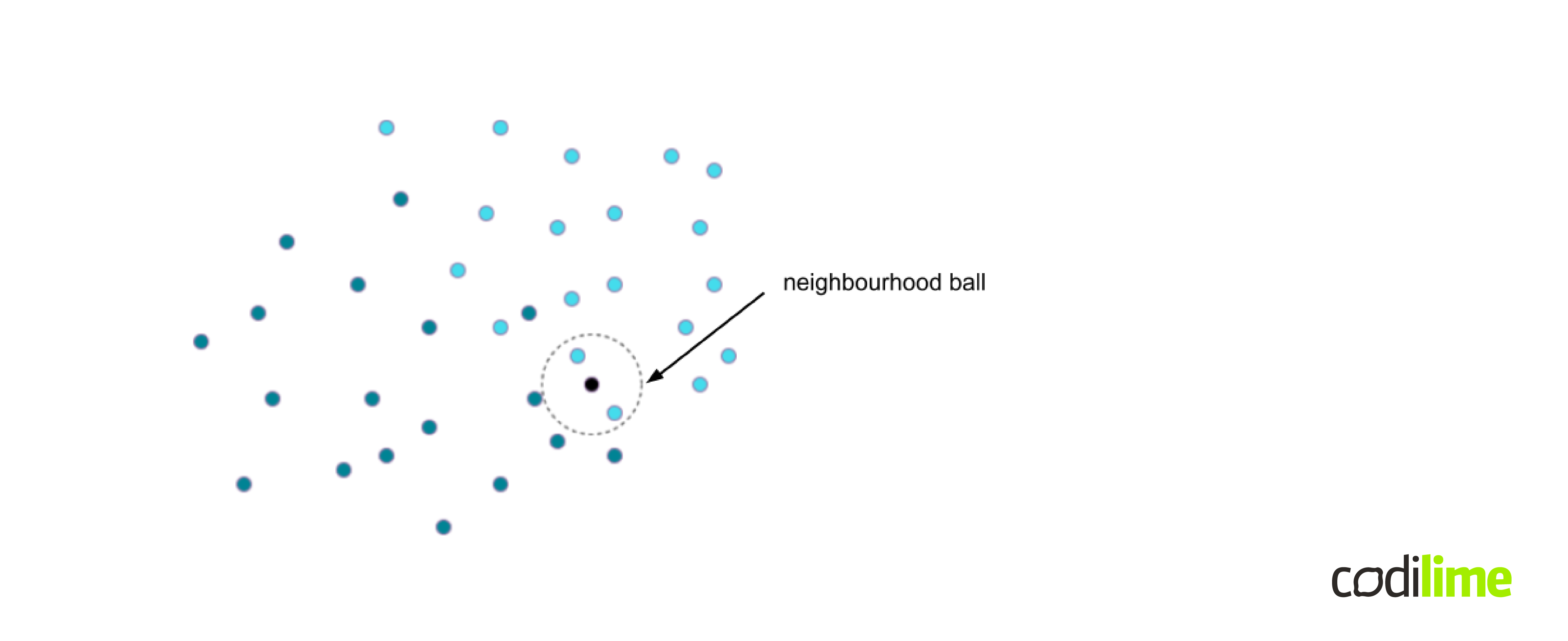
The dark green and blue dots represent the two different classes we are considering. The task is to classify the observation marked on the figure as a black dot of unknown class membership. The algorithm first determines the nearest neighbors of the black point in the training set based on some notion of distance. In the case of the k-nearest neighbor classification algorithm, where k is a user-defined constant, k neighbors are considered and majority voting of classes takes place. The scenario in which k=2 is shown as an example in Figure 6 in the form of a dashed circle and the black dot will be classified as part of the light blue class. A key part of the algorithm is how the distance between observations is calculated. In the context of a time series, we need to find a way to compute the distance between time series to use such an approach. In practice, it is common to use norms such as p-norms (such as Manhattan distance, Euclidean distance, etc.) or the dynamic time warping algorithm. The k-nearest neighbor classifier with dynamic time warping distance is often used as a benchmark solution in various time series classification tasks.
Other approaches that can be used for time series classification are the following: time series forest, proximity forest, rocket algorithm, boss algorithm, MrSQM algorithm and many many others.
Time series anomaly detection
Anomalies are observations that differ from the well-defined concept of normal behavior in the collected data. Very often, these observations carry very significant, meaningful information. As an example, consider anomalies detected in a patient's EEG signal that may indicate some kind of cardiac dysfunction. In the network context, anomaly detection is a field dedicated to finding such abnormal observations and patterns and plays a key role in ensuring reliable network performance.
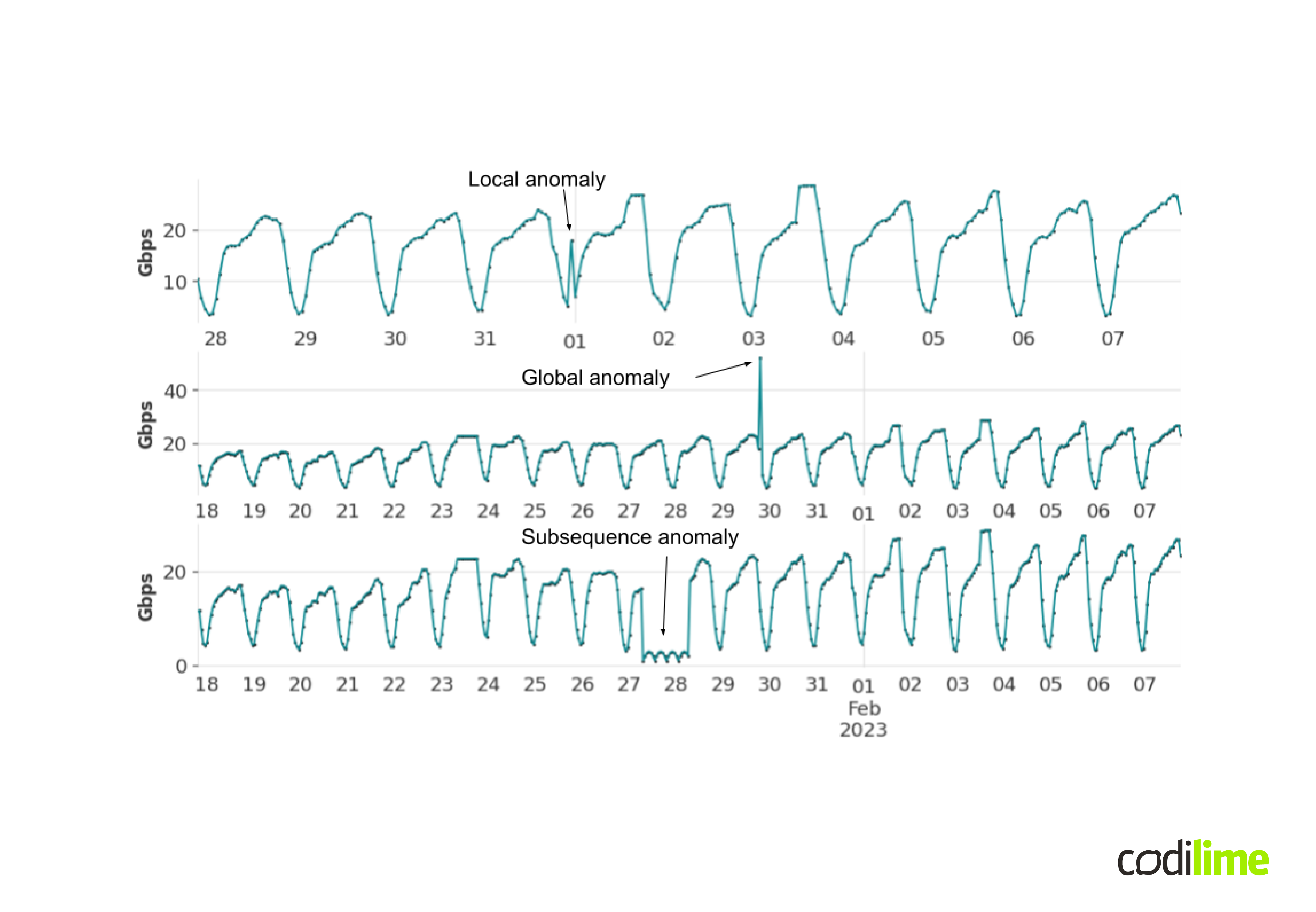
In the context of time series, we can define three types of anomalies, examples of which are presented in Figure 7. The first graph shows a local outlier. This is an observation with the value globally present in the data (equal to around 15 Gbps), but in the context of the moment in time in which it occurs, it is no longer common. The second graph shows an example of a global anomaly, which is an observation of a globally absent value so far. The third graph, on the other hand, shows a subsequence anomaly, which consists of several consecutive observations that create a new pattern in the data.
There are many different approaches to detecting anomalies, most often dedicated to a specific type. An example of a method that can be applied to any type of anomaly is detection using forecasting. The idea is quite simple, you compare the observed signal to previously made forecasts. If they differ to a significant degree, you mark such observations as anomalies. This approach is definitely sensitive to the quality of the forecasts, which should be monitored so that raised alarms do not turn out to be false. Also important is how the forecasts are compared with the actual signal and what it means to "differ to a significant degree" for a given point to be an anomaly. Cooperation with a domain expert to help fine-tune such a solution can definitely play a key role.
Model building challenges
Creating machine learning algorithms in practice is not as simple as it might seem at first glance. There are many hurdles to overcome on the way to creating a useful algorithm. One of the first things to do is data preprocessing, which can, for example, include data cleaning, instance selection, normalization, data coding, transformation, feature extraction, and selection. This part of model building often takes up most of a data scientist's time. As we have already seen, there are many different models/methods for a particular machine-learning problem. They differ in their mathematical perspective towards the problem under consideration, often make different assumptions, and therefore have different properties. Their usefulness depends on the characteristics of the input data, and they differ in the computational resources needed, and in the time it takes to perform calculations. The task of the data scientist is therefore to choose such models/methods that meet these technical as well as business requirements. It should also be remembered that the available methods/models are just tools in the hand of the data scientist, who builds the final algorithm from them. Often, the data scientist's work requires implementing their own proprietary solutions, not just using existing ones. Once again, developing machine learning algorithms is not as simple as it might seem.
Summary
Time series are a type of data that can be used in many different beneficial ways. In this blog post, we've outlined a few of them, illustrating example use cases. Despite significant advances in time series analysis techniques, they remain a major challenge for data scientists. Nevertheless, the benefits that time series analysis brings repay the effort.


