


How CodiLime built a proof of concept that teaches the Kubernetes scheduler what your workloads actually do.
Most of the noise around "AI in the enterprise" right now covers the same ground: a chatbot, a copilot, an agent wired into a workflow. Useful, no doubt. But it is also the shallowest layer of what machine learning can do.
There is a quieter kind of AI/ML work breaking new ground. It runs underneath the platform, on decisions your infrastructure already makes thousands of times a day. And one of the most expensive of those decisions, in almost every Kubernetes estate we see, is also one of the least examined: where to place a workload.
This article walks through a proof of concept CodiLime built for intelligent, ML-driven scheduling in Kubernetes. It is a working PoC on a lab cluster, and it is a clean illustration of where AI implementation expertise creates real value.
The goal is not to replace Kubernetes’ existing scheduling, requests, limits, or autoscaling mechanisms. It is to explore whether learned workload behavior can become an additional placement signal, especially in environments where static resource declarations are intentionally conservative, and workloads show repeatable patterns.
First, what the scheduler actually does
When a request arrives at the kube-apiserver to run a new Pod, something has to decide which node it lands on. That something is the scheduler, and the job sounds simple: find an appropriate node. Underneath, it's a complex multi-stage pipeline.
Pods waiting to launch are queued. First in, first served, unless you've configured otherwise. Then comes filtering, which eliminates nodes that can't host the Pod at all, using rules like taints and tolerations or anti-affinity. The survivors go through scoring, where each remaining node gets a number; a node with more free resources typically scores higher, though many criteria feed in. The highest score wins, and binding launches the Pod there.
Two things matter for the rest of this story. First, scoring is where placement quality is actually decided. Second, and this will become important later, every stage of this pipeline is an extension point. Kubernetes ships standard plugins for each phase, but the framework is open. You can write your own.
The real problem: requests and limits are a guess
Before a workload can be scheduled well, Kubernetes needs to know how much it will consume. You tell it, per container, with two numbers: a request (the minimum resources the container needs to run properly) and a limit (a ceiling, usually set higher to absorb spikes; exceed it and the container gets throttled or evicted). The scheduler aggregates requests per node and uses that to decide what else can fit.
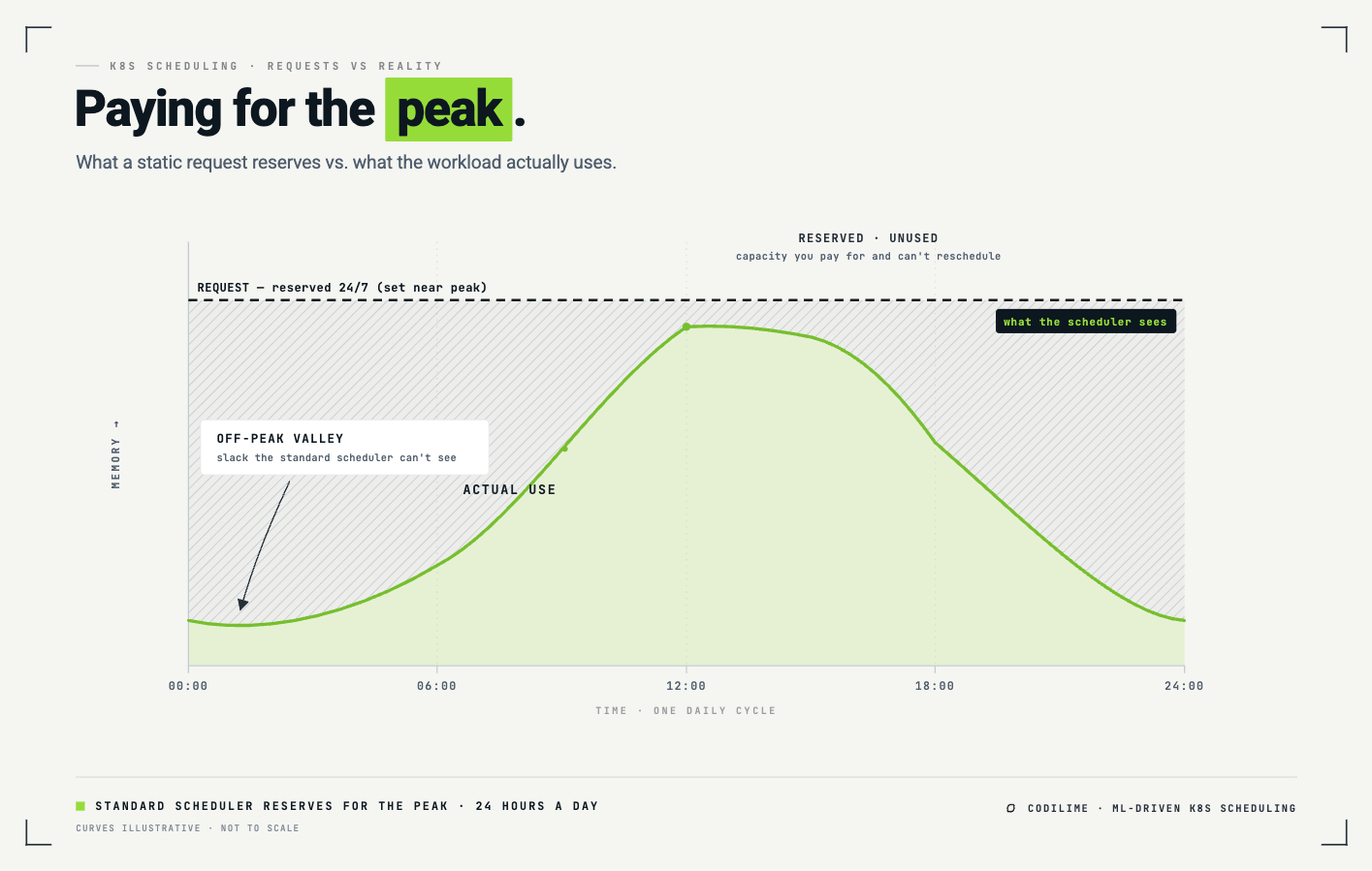
The trouble is that these numbers are static declarations of a dynamic reality. Consider an application whose memory use is cyclic, with heavy use during business hours and light overnight. You have two bad options:
Set the request close to the peak. Now the workload is always safe, but the scheduler reserves peak-sized capacity even at 3 a.m., when the app is barely using a fraction of it. The cluster looks full while sitting half-idle. This is how you end up paying for nodes that are mostly empty.
Or set the request closer to the average. Now the scheduler will happily pack more Pods onto each node, until several of them spike at once, blow past the node's capacity, and you get the overcommitment failure modes: out-of-memory kills, restarts, slowdowns, evictions.
So teams often opt for something in the middle, trading utilization against stability, and re-tuning by hand whenever something breaks. The declared number is a guess, and the cluster pays for the error with wasted capacity.
In many real environments, requests are deliberately overestimated to avoid incidents. That is a rational operational choice, but it also means the scheduler may treat a cluster as full long before the underlying nodes are actually saturated. Autoscaling can add capacity, but it does not fully solve the placement problem if the scale-out decision is based on conservative static declarations rather than observed workload behavior.
The idea: learn the workload, don't trust the manifest
The insight behind the PoC is that this guess can be complemented with a learned model. If you watch what a workload actually consumes over time, you can characterize it, and a characterized workload can often be scheduled more efficiently than one based only on static declarations
That said, learned behavior should be treated as a forecast, not a guarantee. Workload patterns can drift after application releases, traffic changes, business events, infrastructure changes, or shifts in input data. A production implementation, therefore, needs continuous validation, confidence scoring, safety margins, and conservative fallback behavior when predictions become unreliable.
What can you learn? Several distinct things, depending on the workload:
- Cyclic applications reveal a repeating pattern. Detect the cycle, and you can forecast consumption hour by hour rather than reserving for the peak around the clock. In practice, that forecast should include uncertainty bounds or a safety margin, because not every cycle remains stable over time.
- Non-cyclic workloads won't give you a clean pattern, but standard time-series forecasting may still help, and in some cases, you can lean on the statistical shape of the data to bound what to expect. Here too, forecast confidence matters: if the signal is weak, noisy, or based on insufficient history, the scheduler should become more conservative.
- Jobs and CronJobs are a special gift. They spin up concurrent Pods running the same code over different data, so their resource behavior tends to repeat run to run. Learn the signature from historical runs, and you know what the next batch will do before it starts. For new or significantly changed Jobs, the system should fall back to declared requests or class-based defaults until enough runtime history is available.
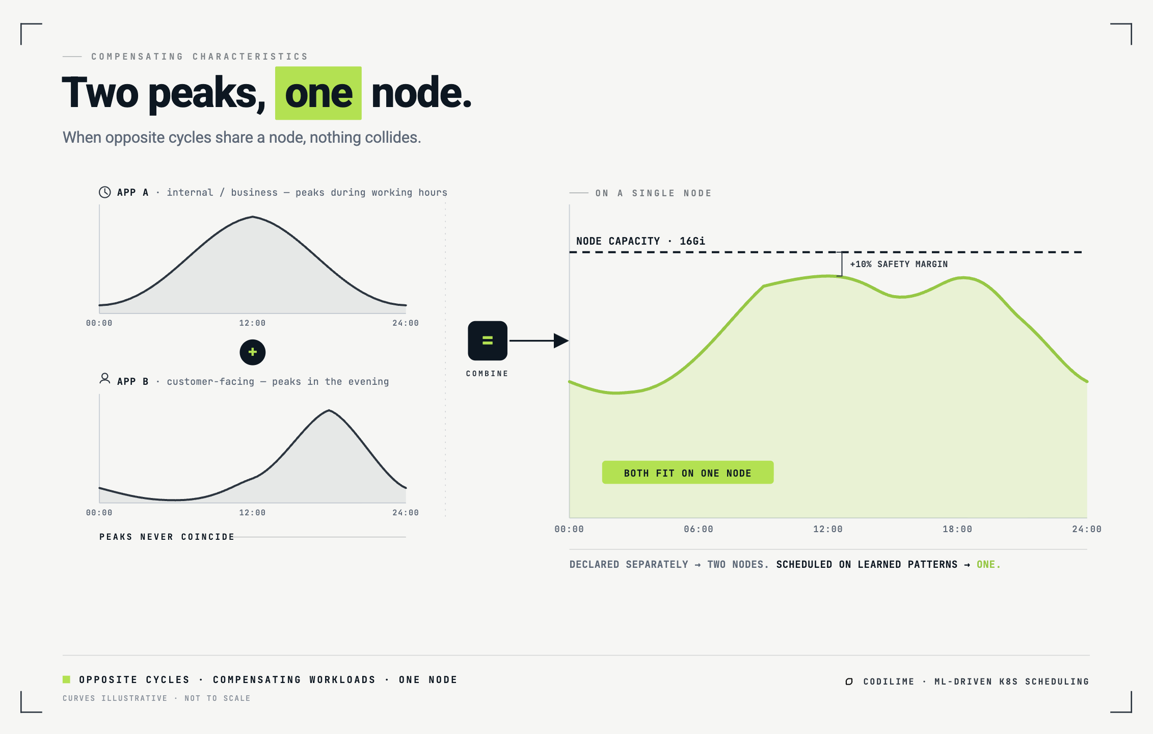
The most intuitive payoff is what our team calls compensating characteristics. Picture two cyclic applications with opposite daily curves: an internal business app that peaks during working hours, and a customer-facing app that peaks in the evening. Scheduled by declaration, each demands its own peak-sized reservation, so they land on two nodes. But their peaks do not coincide in the observed historical window. A scheduler that knows both patterns can place them on a single node, because their combined consumption is forecast to remain below its capacity. Two nodes' worth of declared demand, served by one.
In a production system, this decision should be continuously re-evaluated. Previously complementary workloads can become correlated after release changes, traffic shifts, incidents, marketing events, or expansion into new time zones.
The same logic governs Jobs. If you've learned a Job's consumption pattern and you're forecasting a node's near-future load, you can simply check: does accepting this Pod, right now, push us over capacity? Sometimes the answer is no, wait. A little later, in the application's off-peak valley, the same node can absorb two such Pods at once.
Distilled to three steps, intelligent scheduling means: learn the consumption pattern of each workload, forecast the future utilization of each node, and select the best node for an incoming workload based on those forecasts. That is exactly what the standard scheduler does, except it scores on declarations, and this scores on learned reality. That one substitution is the whole difference.
More precisely, it scores on learned reality plus policy constraints. Forecasts should not replace hard limits, existing Kubernetes rules, affinity and anti-affinity, taints, quotas, or operational guardrails. They should act as an additional signal in the placement decision.
This complements autoscaling rather than replacing it. Autoscalers decide when more or fewer resources are needed; the scheduler decides how well available resources are used. If requests are inflated for safety, autoscalers may add nodes while existing ones still have usable capacity. Forecast-aware scheduling helps reduce that gap by improving placement before scale-out is needed.
How we built it
The PoC keeps the learning and the scheduling cleanly separated, connected through the scheduler's own extension points.
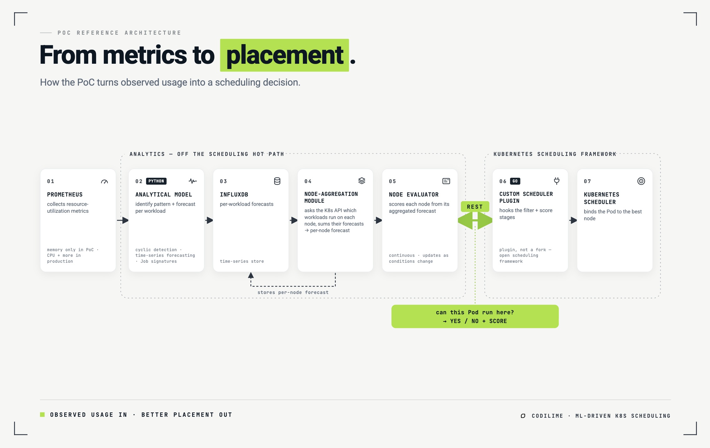
It starts with metrics. Prometheus collects resource-utilization data from the cluster. An analytical model pulls those metrics, identifies the consumption pattern for each existing workload, and forecasts its future use. Those per-workload forecasts are written to InfluxDB, a time-series database.
A second analytical module turns per-workload forecasts into per-node ones. It asks the Kubernetes API which workloads are running on each node, pulls their individual forecasts from InfluxDB, and produces an aggregated forecast per node, which it stores back in the database.
A node evaluator then reads those aggregated forecasts and computes a score for each node continuously, as conditions change. This is where "which node is the best home for this Pod right now" gets answered, using forecasts instead of static reservations.
The last piece connects all of this to Kubernetes itself. Because the scheduling framework is open, we wrote a custom scheduler plugin in Go that hooks into the filtering and scoring stages and talks to the node evaluator over a REST API. When a Pod needs a home, the scheduler asks the evaluator, per node: can this Pod run here, and what's the score? The evaluator answers from its forecasts; the scheduler places accordingly and triggers a forecast update.
In a production design, this control-plane-adjacent path would need strict timeouts, health checks, degraded-mode behavior, and fallback to standard scheduling logic if the evaluator, forecast store, or analytics pipeline becomes unavailable. The scheduler should never block indefinitely or make unsafe placement decisions because an external scoring component is unhealthy.
No fork of the scheduler, no patched core, just a plugin that the framework already provides.
The full stack: Kubernetes as the platform; Prometheus, Grafana, and Grafana Loki for observability and logs; InfluxDB for time-series storage; Python for the analytics and ML; Go for the scheduling plugin.
The quality of the placement decision is also bounded by the quality of the telemetry. Missing metrics, scrape gaps, delayed data, low-resolution aggregation, or incorrect labels should reduce model confidence and trigger conservative scheduling behavior.
The demo: packing Jobs into the valleys
To show this working, we ran a use case called efficient Job execution.
The lab cluster: four worker nodes, 16Gi of memory each. On them, four cyclic applications (one replica apiece) with different memory profiles ranging from roughly 2G to 10G. Into that running environment, three batch Jobs are submitted, each needing 50 Pod completions, each Pod consuming up to 4G, and the goal is to finish all three as fast as possible, at maximum concurrency, without a single out-of-memory kill or restart. The three Jobs differ by shape: a flat Job (steady memory throughout), a high-start Job (heavy early), and a low-start Job (light early, heavy late).
What would normally happen in a standard scheduler, working from peak-sized requests, could only fit a single Job Pod per node at a time because it has no way to know there's slack hiding in an application's off-peak valley. The intelligent scheduler does know. It recognizes each application's cycle and each Job's signature, and it slots Job Pods into the troughs: more Pods during the valleys, fewer during the peaks, staying under capacity in the observed PoC scenario.
A production implementation would need additional safeguards for unexpected spikes, correlated workload behavior, telemetry gaps, and forecast error.
The demo's dashboards let you watch each stage happen. One shows the analytics correctly picking up the applications' cycles; another shows the distinct memory shape it learned for each type of Job. A third surfaces the live back-and-forth between the scheduler and the node evaluator: the scheduler asking whether a given Pod can run on a given node, the evaluator answering yes or no, and returning a score. And one console does nothing but watch for Pods killed by out-of-memory errors. It stays empty the whole run. That empty console is the point of the demo: the cluster is being packed more aggressively, without observed OOM kills or restarts during the run.
The result was that completing the three Jobs took 16 minutes with the intelligent scheduler versus 37 minutes with the standard one in this lab scenario**.** That's almost 2.5× faster. Real-world gains will depend on workload repeatability, telemetry quality, cluster size, workload mix, policy constraints, and the level of safety margin required.
See for yourself in the video here:
What it costs, and what it saves
We'll keep this balanced, because the costs are real.
The benefits come in two forms. The obvious one is capacity: if you can lift a cluster's real utilization from 30% to 60%, you may be able to host the same workloads on significantly fewer worker nodes, which can translate into infrastructure savings. The quieter benefit is operational: a lot of the manual work around cluster capacity planning, dimensioning, safety margins, and tuning requests and limits gets absorbed by the system, so administration gets easier and less reactive.
The exact business impact depends on whether the organization can actually decommission nodes, avoid future capacity expansion, or reduce cloud spend after accounting for analytics overhead, high availability, observability, and operational complexity.
The costs are equally real. You're adding software components and the compute to run them. The analytics aren't free, and their overhead scales with the number of deployments, Jobs, and patterns being modeled. On a 70-node cluster, doubling utilization might free ~35 nodes; subtract the nodes you spend on analytics, and you may still come out ahead, but the math only works at scale. On a small cluster, the overhead can eat the gain.
This points to where this belongs first: large development environments are the strongest candidates. They tend to be over-provisioned, and they're full of repeatable patterns, which is exactly the raw material the learning side feeds on.
They are also typically more tolerant of controlled experimentation than business-critical production clusters, while still large enough for utilization gains to outweigh the overhead of the analytics stack. Production use should follow a more cautious path: shadow scheduling, canary rollout, conservative safety margins, policy-based exclusions, and clear rollback procedures.
Beyond scheduling
Efficient Job execution is one use case, but the same learned-characteristics foundation supports others: intelligent autoscaling of Deployments, and trend analysis that predicts upcoming out-of-memory conditions before they hit. Once you have a model of what workloads actually do, scheduling is just the first thing you can do with it.
The same foundation could also help tune resource recommendations, detect drift between declared and actual usage, and identify workloads whose behavior has changed enough to require human review or policy adjustment.
The takeaway
The Kubernetes scheduling framework is open and built for exactly this kind of extension. We used that to insert AI/ML where the scheduler is otherwise flying blind between what a workload was declared to need and what it actually consumes. The result, in the PoC, was meaningfully tighter packing without observed OOM kills or restarts during the demo scenario, and a path to fewer nodes and less manual cluster work, especially on large development clusters.
Turning this into production-grade scheduling would require confidence-aware placement, drift detection, fallback to conservative scheduling, and progressive rollout controls. Static requests, limits, autoscaling, and policy constraints remain necessary. The opportunity is to add a learned placement signal on top of them, especially in large clusters where requests are intentionally conservative, and workload behavior is repeatable enough to create usable forecasts.
There's no chatbot in this story, and that's the point. The differentiation isn't a model call; it's the engineering.


