Long-term time series forecasting: an insight into the methods

Time series forecasting is the prediction of the future values of a time series (you can find our blog post about time series here) based on its historical values. It owes its practical importance to its ability to make optimal decisions for a future that has not yet arrived. For example, it gives the ability to react in advance and prevent problems that would arise in the future, which certainly reduces the cost of handling them. To illustrate this, we present an example use case from the IP core network domain. 

Long-term traffic forecasting is a mandatory task delivering necessary data for the network analysis of future traffic conditions. Forecasting traffic, we can evaluate when the network is expected to be congested, which network elements will have insufficient packet forwarding capacity, and when the network will not be able to carry the whole traffic if any failure from the assumed scenarios occurs. The complete use case was presented on the webinar      . 

In this article, we describe the use case and reasoning for long-term traffic forecasting, next we focus on the methods we used, and discuss alternative approaches and challenges to overcome.

A practical use case for time series forecasting

Consider an example  IP core network  topology presented in Figure 1.

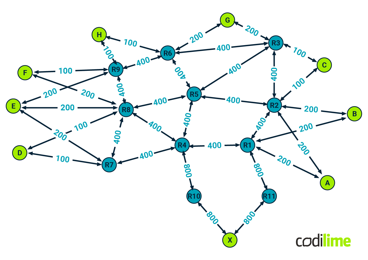
Core routers colored dark green and labeled R1 through R11 forward traffic between any pairs of edge routers colored lime green and marked A through X. The edge routers handle traffic coming from other segments of the provider’s network, e.g. from an aggregation network, BNG (broadband network gateway) devices, mobile packet core, or even very high-speed access devices in some cases. This depends on how the given network is laid out. The graph represents an example network topology and the labels on the edges show link capacities expressed in Gbps. Each link may consist of several aggregated links underneath. For example, if a link has a capacity of 400 Gbps, it may consist of four 100 Gbps links. 

We assume that the following types of failures may occur in the considered network:

• a single node failure - when one of the core routers is broken; it is worth noting that in our scenario this also means that all links adjacent to the failed node become inactive in the network, 
• a single link failure - when the link between two given routers becomes fully inactive   (e.g. due to some issues occuring in the underlying transport network layer that handles a physical connection for the considered IP core routers),
• a partial link failure - when only part of an aggregated link between two given routers becomes inactive (e.g. due to damage to one of the router’s interfaces); the link is still up but its capacity has decreased.

We assume that only single failures are to be considered as part of the further analysis, i.e. those in which a single element (a router or a link) is the source of the failure at a given moment. Other cases, i.e. multiple failures, although possible, are much less likely to happen.

It is worth noting that when a single node failure or a single link failure occurs, it triggers routing recomputing in the network. This is because the network topology graph has changed. This is not the case when a partial link failure takes place.

Of course, we want the considered network to be resilient to any of the above-mentioned failure scenarios. Typically, this is achieved by applying a certain level of over-provisioning in terms of network capacity. This means that the capacity of the network is enough to carry all the traffic not only under standard conditions but also when different types of failures occur. 

Additionally, you need to know that traffic volume is changing over time, most likely with an increasing trend over some period of time (e.g. over several months) so network capacity configured at any given moment might be insufficient in the future. Here the question arises: how to determine if the network still has an ability to be resilient in terms of congestion (also taking into account possible failure scenarios)?

A need for traffic forecasting

Let’s address the problem of future network overload. First of all, we want to know in advance when the network may be overloaded; i.e. the assumed level of resilience is not guaranteed. Also, we want to know exactly which network elements will suffer from lack of capacity. With this knowledge, it is possible to react in advance and prevent future lack of capacity problems and their consequences. 

One possible solution is to increase in advance the capacity of the link(s) for which we anticipate future congestion. The question is: how much should link capacity be increased? To obtain future network loads, we forecast the bit rate of E2E (end-to-end) traffic between any pair of edge routers. These flows are in the form of time series. For example, the topology shown in Figure 1 has nine edge routers, so we need to forecast 72 time series to fully monitor the load in the network. In Figure 2, an example traffic flow from router X to router E is presented. The top graph shows the traffic flow (i.e. a flow bit rate expressed in Gbps) from a few months' perspective. You can clearly see a strongly increasing linear trend here. 

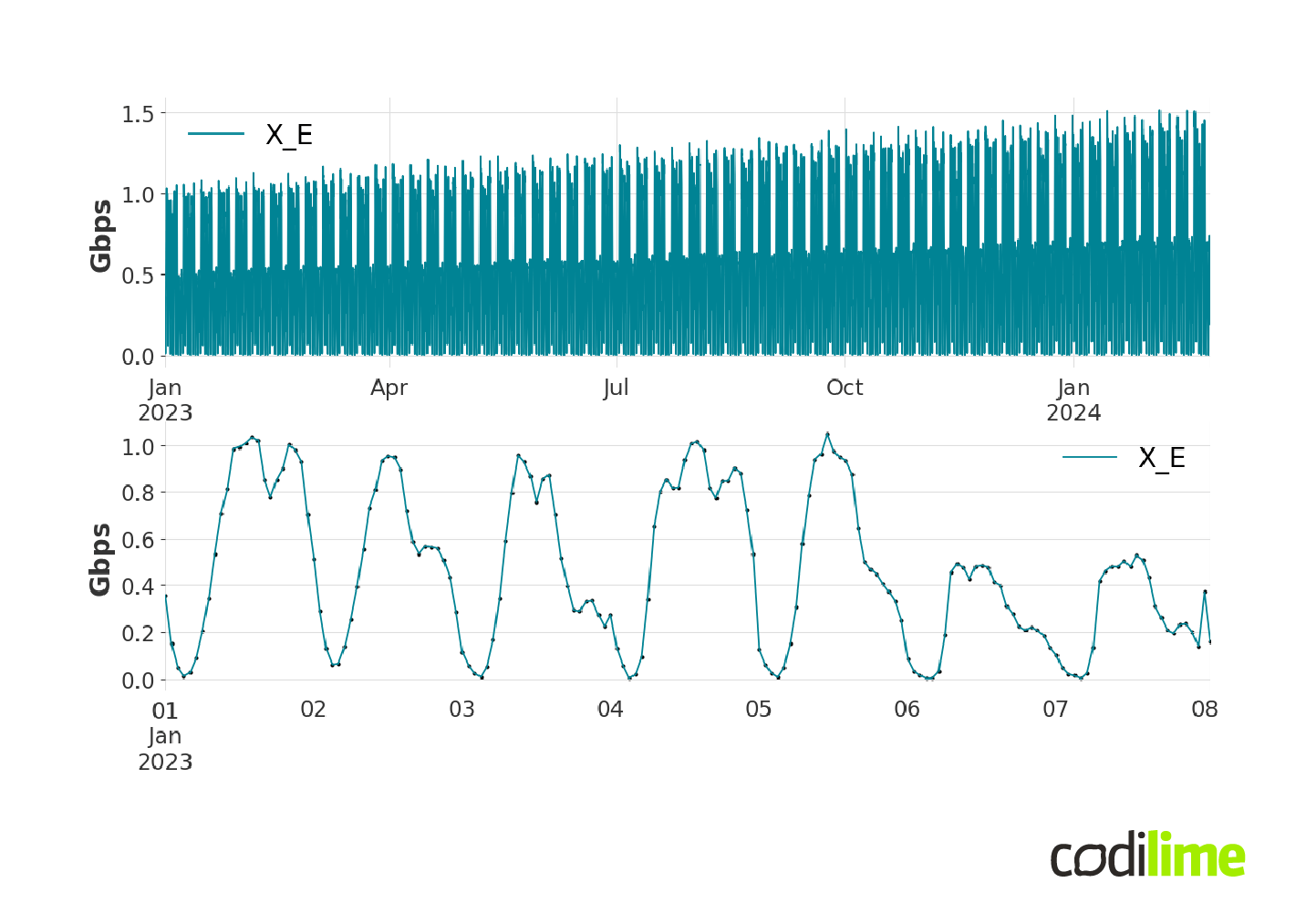
The second graph in Figure 2 presents a weekly perspective for the same flow. The dots represent a single measurement taken every hour - this is the frequency of the measurements, the size of which greatly affects the time needed to obtain forecasts. At this point, it is useful to define the forecast horizon we are aiming for.

Typically, network expansion plans are made annually, so we set the forecast horizon at this value. Since the measurement frequency is one hour, the forecast should be 24 (hours in a day) x 365 (days in a year) = 8760 points. That is a lot of points to forecast! Imagine forecasting the air temperature for the next year with hourly resolution. This is a very difficult challenge. The task of time series forecasting for such a large horizon is called long-term time series forecasting. Please note that for the considered network we need to forecast 72 time series at the same time to monitor future network loads, and this number is growing with the number of edge routers. This means that our forecasting solution has to be quite general and provide good quality forecasts for different input data.

ML processing pipeline for  traffic forecasting: an example approach

Figure 3 presents an example ML processing pipeline for long-term time series forecasting.

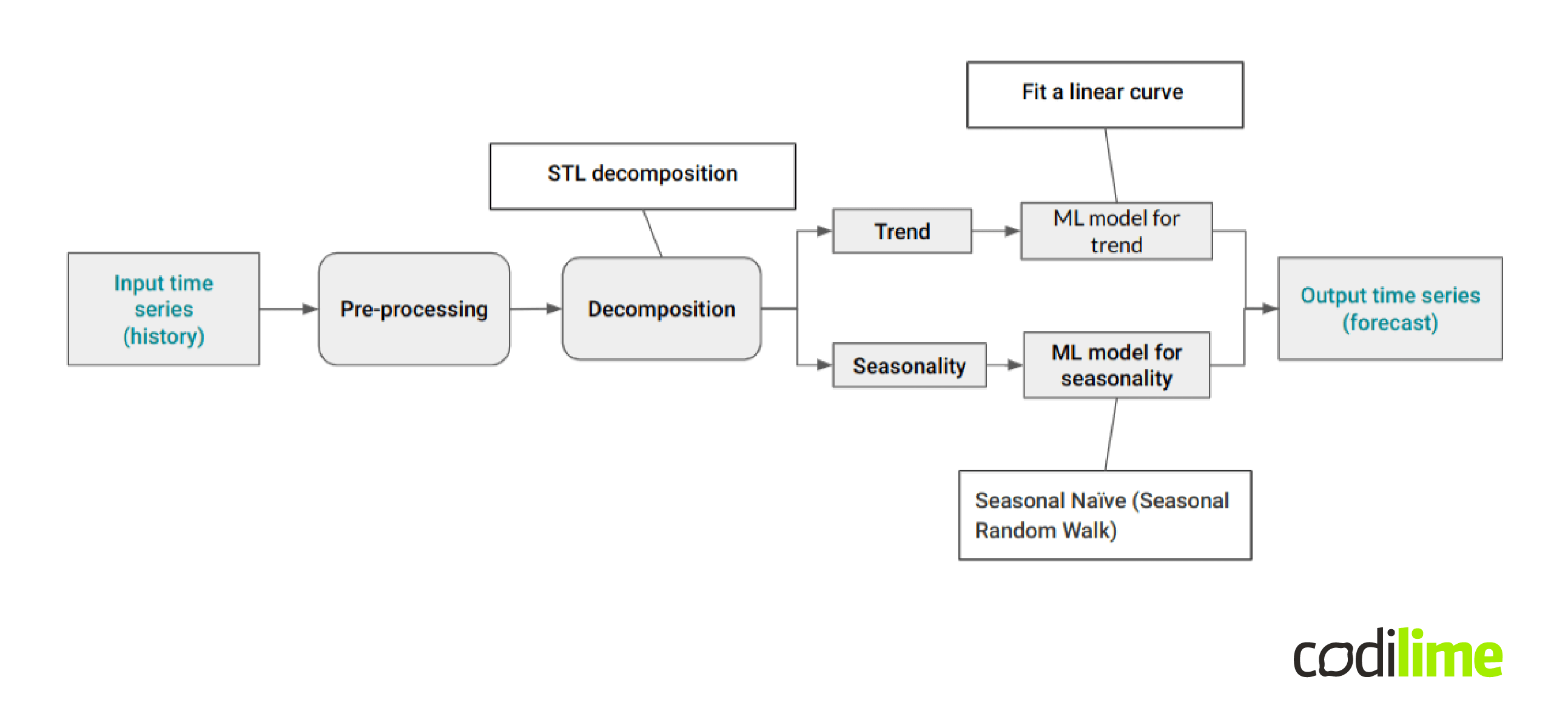
A single time series is taken as input. The next step is data preprocessing, which can include:

• filling data gaps (imputation of missing data in the measured time series), 
• outlier detection and handling (what to do with data points that differ significantly from other observations), 
• noise filtering,
• and other data preparation manipulations (e.g. variance stabilizing transformations, feature engineering, and many others).

We do not go into the details of preprocessing in this blog post.

After data preprocessing, we move on to the actual time series forecasting part.  We decided to use a decomposition approach, and selected STL decomposition      , where  STL stands for "seasonal and trend decomposition by Loess". The STL method decomposes the input time series $Y_t$ into three components:

$Y_t = S_t + T_t + R_t$, where

$S_t$ is a seasonal component that represents seasonal-cyclic behavior of a time series, $T_t$ is a trend component which correspond to long-term behavior of a time series, and $R_t$ is a remainder component which is the part of the signal that was not included in either of the two other components. In Figure 4, we have presented a decomposition of an example signal to make it easier to understand the meaning of each component.

STL is a filter-based procedure that works recursively. This means that at each step the algorithm updates the results obtained in the previous step. Due to the multitude of steps it involves, we have omitted the full details of the procedure. Nevertheless, it has gained practical importance due to its ease of use and speed of calculation, even for long time series. 

It is also possible to use STL decomposition as a multiplicative decomposition method using the log-exp transformation trick. If we want to decompose input signal $Y_t$ into

$Y_t = \overline{S_t} * \overline{T_t} * \overline{R_t}$

we first apply log transform to the input signal and then additive STL decomposition to the log-transformed signal:

$logY_t = log(\overline{S_t} * \overline{T_t} * \overline{R_t}) =$ $log\overline{S_t} + log\overline{T_t} + log\overline{R_t}$,

and to obtain multiplicative decomposition components we just apply the inverse function of a logarithm - exponential function - to those obtained from STL decomposition. Note that the logarithm can be applied to values strictly greater than 0! Multiplicative decomposition is very useful when seasonal variations change over time. 

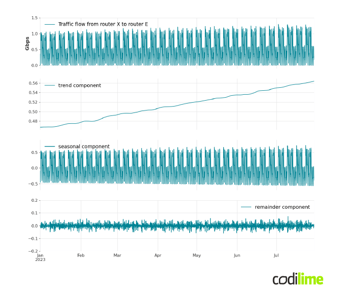
As an example, Figure 5 shows the STL multiplicative decomposition for the traffic flow from router X to router E. The reason why we should use multiplicative decomposition instead of additive decomposition for this signal will be clear in a moment.

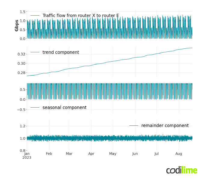
The first graph shows an input signal that clearly exhibits strong seasonal behavior with a periodicity of seven days. This is quite typical for aggregated traffic flows carried by IP core networks when weekly patterns are quite regular. The periodicity is the crucial parameter for the decomposition method. We discuss how to detect it if it cannot be easily observed from data later in the next part of this blog post. The linear upward trend of the entire traffic is also noticeable, but in general traffic trends can have more complex curves. 

The next three graphs present the result of the STL decomposition of this signal.  The first component represents the trend, which, as we expected, is a linear increase, but with slight fluctuations. The next one is the seasonal component, which presents cyclical changes in traffic over the week. The last component is the reminder, which presents the part of the signal that was not included in either of the other two components.

According to the scheme shown in Figure 3,  after decomposing the time series, we forecast each component individually, typically excluding the remainder component from our predictions. This remainder is often assumed to represent a small or negligible portion of the overall signal, approximated as a constant (close to 0 in additive decomposition, close to 1 in multiplicative decomposition), hence considered ignorable for forecasting purposes. Nevertheless, there are scenarios where it might be justifiable or beneficial to include forecasts for this component as well.

In order to forecast the trend for the considered time series we can use a linear function. This means that we limit our model only to data that exhibit linear trend behavior. In order to forecast the seasonal component, the seasonal naïve model can be used, which is often good enough and a fast solution when seasonal patterns show a high level of regularity. The method divides the historical data into blocks of period length, evaluates an average block best fitted to the historical data and uses it as a repeated pattern for forecasting. The final forecast is the product of the forecasts of each component (addition in the case of additive decomposition). Such an approach can be found in the following code:

from sktime.forecasting.trend import STLForecaster,PolynomialTrendForecaster
from sktime.forecasting.base import ForecastingHorizon
from sklearn.linear_model import LinearRegression
from sktime.forecasting.naive import NaiveForecaster
from pandas import Timedelta
from numpy import log, exp, arange

forecasting_horizon=Timedelta('1y')
seasonal_length=Timedelta('1w')
data_frequency=Timedelta('1h')

seasonal_length_int=int(seasonal_length/data_frequency)
model=STLForecaster(sp=seasonal_length_int,
                    forecaster_seasonal=NaiveForecaster(sp=seasonal_length_int,
                                                        strategy='mean'),
                    forecaster_trend=PolynomialTrendForecaster(LinearRegression()))
model.fit(log(train_set))

values_forecasting_horizon=arange(1,int(forecasting_horizon/data_frequency),dtype='int')
fh=ForecastingHorizon(values=values_forecasting_horizon,is_relative=True)
forecasts=exp(model.predict(fh=fh))

First the necessary libraries are imported: 

from sktime.forecasting.trend import STLForecaster,PolynomialTrendForecaster
from sktime.forecasting.base import ForecastingHorizon
from sklearn.linear_model import LinearRegression
from sktime.forecasting.naive import NaiveForecaster
from pandas import Timedelta
from numpy import log, exp, arange

Next, we specify the length of the forecasting horizon, the length of the seasonal component period and the gradation of the input data.

forecasting_horizon=Timedelta('1y')
seasonal_length=Timedelta('1w')
data_frequency=Timedelta('1h')

Then, an instance of the STLForecaster from the sktime library is created.

seasonal_length_int=int(seasonal_length/data_frequency)
model=STLForecaster(sp=seasonal_length_int,
                    forecaster_seasonal=NaiveForecaster(sp=seasonal_length_int,
                                                        strategy='mean'),
                    forecaster_trend=PolynomialTrendForecaster(LinearRegression()))

We specify the period length - sp - to be 7 days, and also the forecasting models for the trend (PolynomialTrendForecaster) and seasonal components (NaiveForecaster). 

Next we fit the model to the input data (train_set) transformed logarithmically. 

model.fit(log(train_set))

Finally, we create a forecast from the model and perform an exponential transformation to receive final forecasts.

values_forecasting_horizon=arange(1,int(forecasting_horizon/data_frequency),dtype='int')
fh=ForecastingHorizon(values=values_forecasting_horizon,is_relative=True)
forecasts=exp(model.predict(fh=fh))

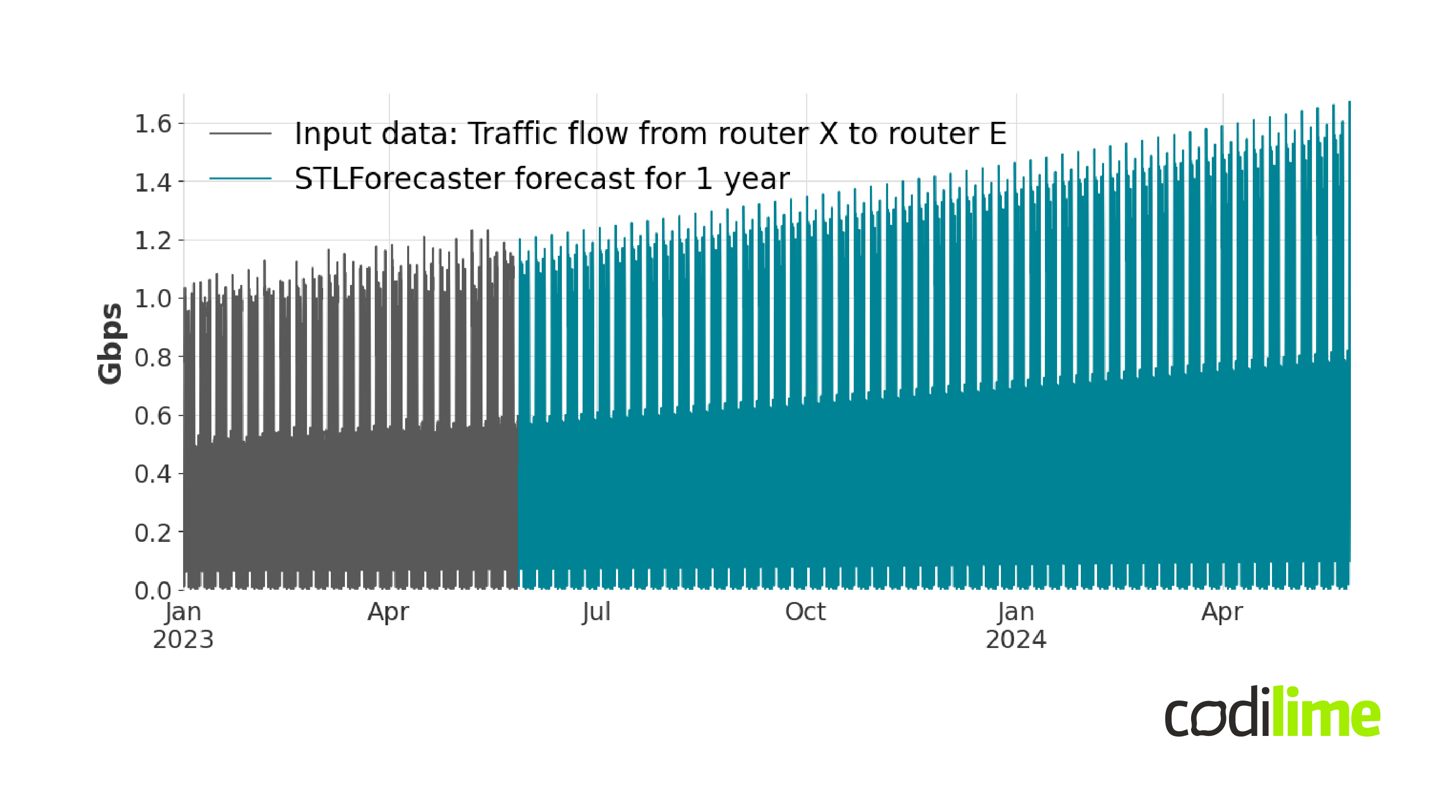
In Figure 6 the annual forecast for the traffic flow from router X to router E has been presented.

If you would rather use the additive version of decomposition you would receive the following forecast:

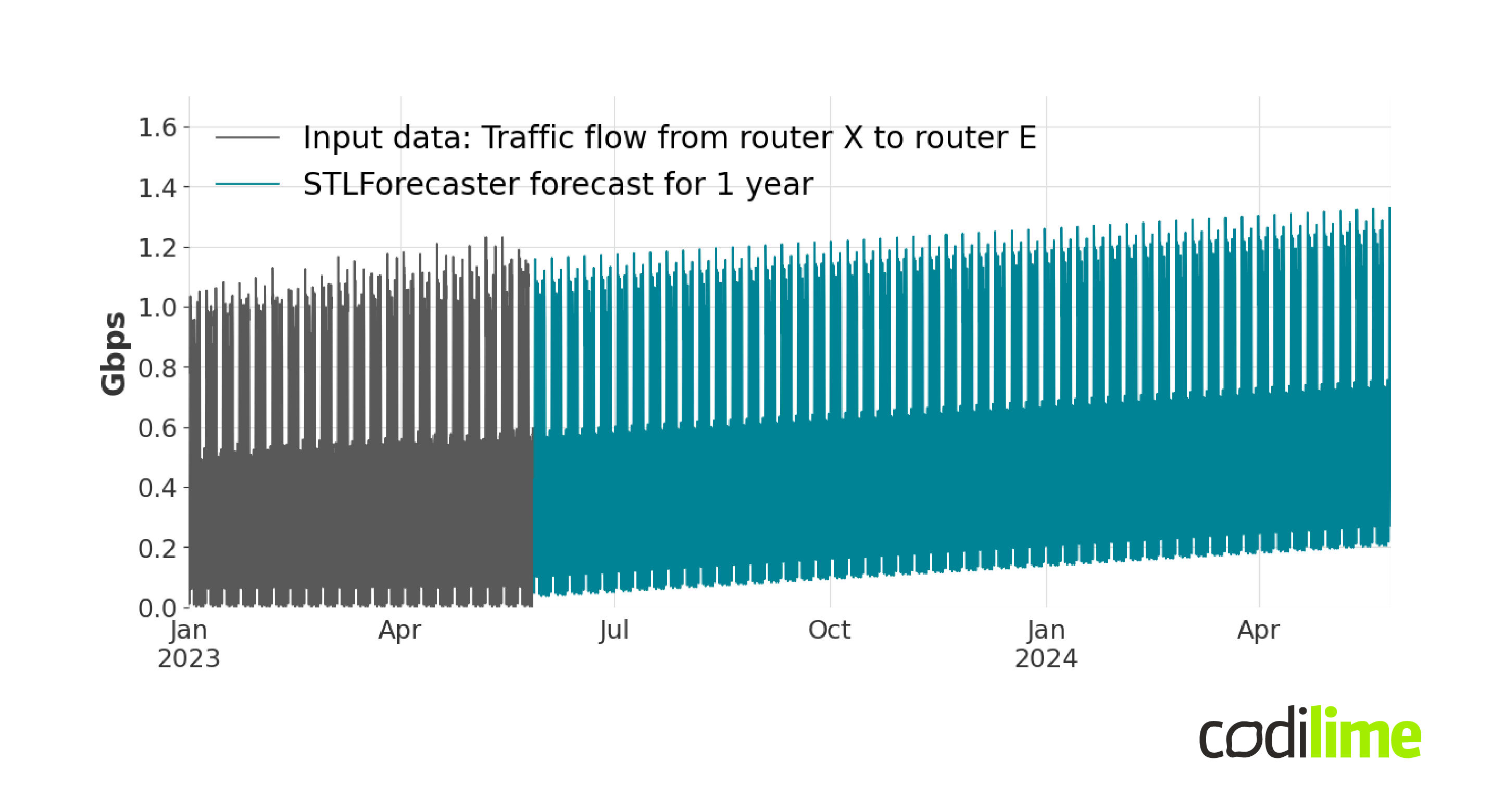
Figure 6 and Figure 7 show quite different forecasting results and the results of additive decomposition seem to be less fitted compared to the historical data. 

In the additive model, the seasonal variations are additive to the overall trend, and their magnitude remains constant over time. This can be seen in Figure 7. The multiplicative model assumes that the seasonal component is proportional to the trend component. This means that the seasonal variations are multiplicatively applied to the overall trend, and their magnitude can change over time (Figure 6).

Now, imagine that our time series database contains both signals for which the multiplicative model is more suitable, and signals for which the additive model is more favorable. In order to automatically determine the most suitable decomposition method for a given input signal, we can employ a validation process. Based on the known historical data, we can apply two models with different decomposition methods to predict the signal (typically with a shorter forecasting horizon) up until the end of the known data. By comparing the predicted values to the actual signal, we can dynamically select the more accurate decomposition method and use it for the subsequent long-term forecasting process, which utilizes the most recent historical data.  As a comparison criterion we can use the MAAPE score

$MAAPE(\{y_t\}, \{\widehat{y_t}\}) =$ $\frac{1}{N}\sum_{t=1}^{N} arctan(|\frac{y_t-\widehat{y_t}}{y_t}|)$,

where $y_t$ is the actual time series value at time t, $\widehat{y_t}$ is the model forecast and N is the number of observations in the compared time series. Formula shows that it is the relative error $(|\frac{y_t-\widehat{y_t}}{y_t}|)$ scaled by the inverse tangent. Its big advantage is that it always takes values from -$\frac{π}{2}$ to $\frac{π}{2}$ (or with a little manipulation from 0 to 1) regardless of the signals being compared. Which makes it a scale-free criterion. 

At the beginning of our analysis, we assumed that the period length is known and equal to one week. What if there are signals with different period lengths in our database? In this case, we must use a method that will determine the period of the seasonal component automatically. We can, for example, treat the period of the seasonal component as an unknown and determine its optimal value using validation as well. Another option would be to use more advanced techniques like time-frequency analysis or periodogram analysis. In this blog post, we do not go into the details of this issue, but we want to emphasize its importance. 

What if a time series has a more complex trend curve than the assumed linear model. And what if the assumed seasonal naïve model is too simple to model a seasonal component with the required accuracy?

An alternative approach to forecast trend and seasonal components

Figure 8 below shows the result of STL multiplicative decomposition for three different signals from the database.

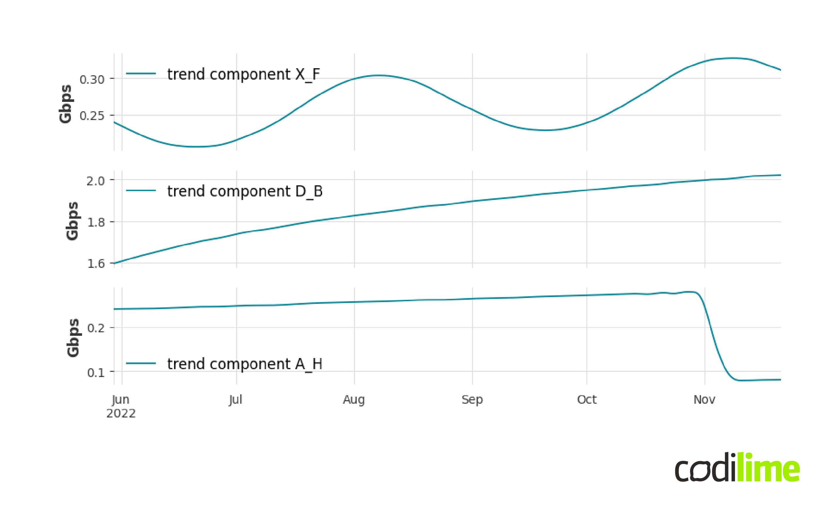
At first glance, fitting a simple linear curve seems inappropriate for each case. The first trend line shows a periodic structure, the next example is a curve showing logarithmic growth, and for the last curve a trend-change point can be observed. The linear curve model is not suitable for these cases. Moreover, these are just a few examples of the complexity you can encounter with trends. Therefore, we need to use a model with greater generalization power that can describe much more complex trends than a linear curve. A good example of such a model is a Gaussian process      , a nonparametric supervised learning method. This is implemented in the gpflow       library. To create an instance of this class we need to specify the mean function and the kernel function (the crucial parameter of a Gaussian process):

from gpflow.models import GPR
from gpflow.kernels import Linear
gaussian_process = GPR(data=(x, y), kernel=Linear, mean_function=None).

Usually the mean function is set to zero (that is why mean_function=None), and in this case the choice of the kernel function fully determines the properties of the Gaussian process. The kernel function essentially determines the distance between two data points and there is a great deal of freedom in its selection. In the presented example we use the linear kernel. However, there are much more commonly used kernels, like: constant kernels, Matérn kernels, periodic kernels, change points kernels, etc. It is also possible to create a custom kernel function. Choosing the kernel needs to be done carefully in terms of making forecasts. 

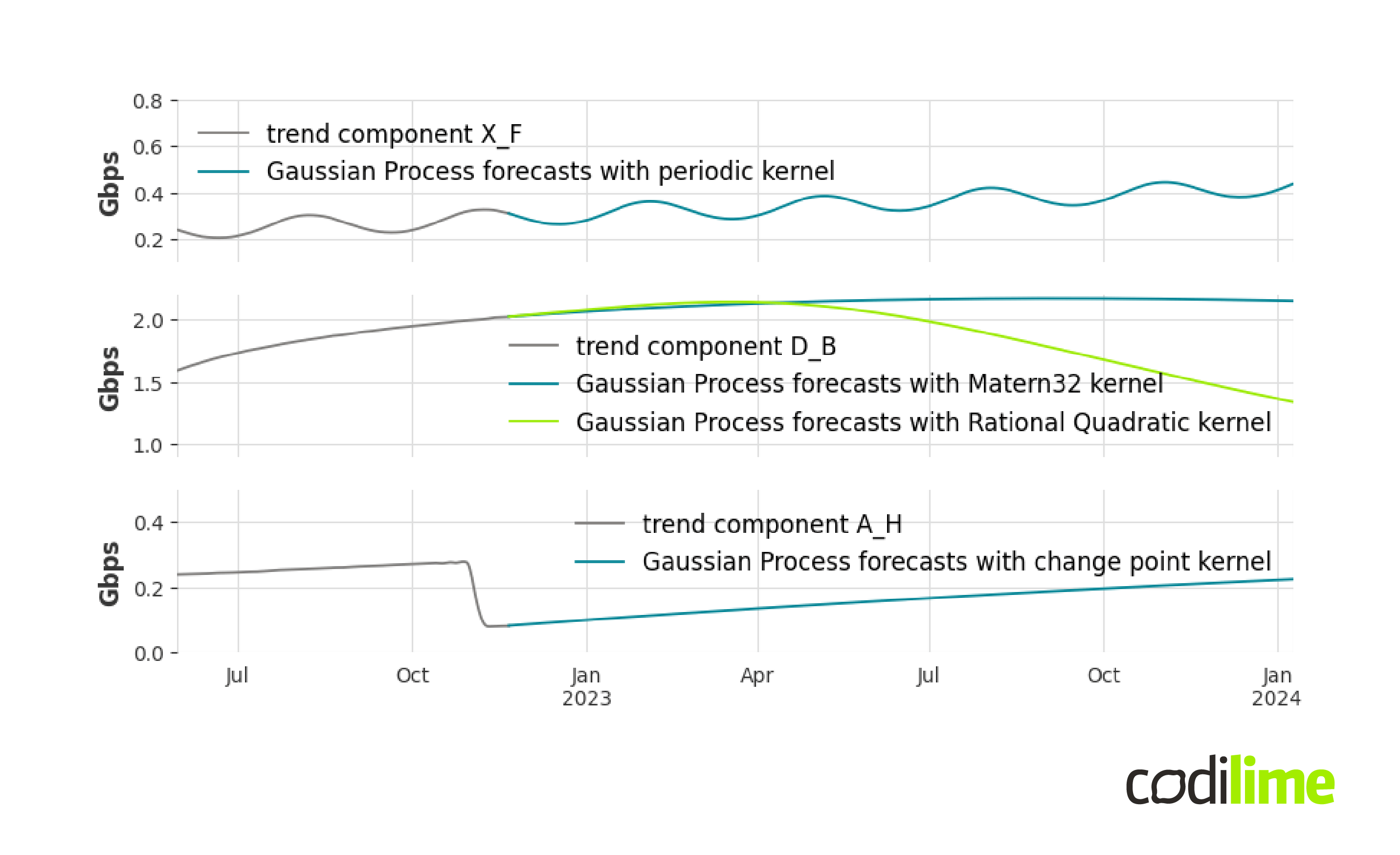
Figure 9 shows forecasts for trends in Figure 8 determined by Gaussian processes with different kernels. In the second chart we decided to show two forecasts obtained from models with different kernels: Matern32 and Rational Quadratic. The question arises which forecast represents the more likely scenario; which is hard to answer in the general case.

Another extension that can be made to the proposed pipeline is to use a more sophisticated model for the seasonal component. A good example is the TBATS       (Trigonometric seasonality, Box-Cox transformation, ARMA errors, Trend and Seasonal components) model. The TBATS model is inspired by exponential smoothing methods but we won't go into details as the model formulas are quite complicated. Nevertheless, TBATS has strong advantages. First of all, it allows a signal to have several seasonalities at the same time and to have non-integer valued periods, and the seasonality is allowed to change slowly over time.

Challenges in long-term time series forecasting

Long-term time series forecasting, by definition, should be considered a challenging task. Long-term means that we have to forecast many values in the future, and the more we have to forecast, the more difficult it is. It is often expected that the model will have high generalization power; i.e. it will be able to forecast (with satisfactory quality) time series with different statistical characteristics. This poses another challenge, as each method has its limitations.

In this blog post, we have not addressed in detail the important issue of data preprocessing, which often takes up most of a data scientist's time. It is worth remembering that improper input data preparation can significantly - i.e. negatively - affect the quality of the forecasts. 

Another important issue can be the optimal choice of the history size for model training which can significantly affect the training time and the quality of the forecasts. In the case of a database with a large number of time series, it may be that using one model is not enough and several ones should be used. This is where the problem of automatic selection of the most promising model or mixing of multiple forecasts comes in. If it is necessary, you must also consider the issue of retraining the model and hyperparameters search. Long-term time series forecasting is not as simple as it might seem.

Summary

In this blog post, we discussed the problem of long-term time series forecasting. We presented an example pipeline for this task, with both simple and more advanced models for trend and seasonal component forecasting. 

We have identified the key challenges and issues related to this complex problem. It takes a lot of effort to make long-term forecasts, but good decisions based on them can be worth it.