Network ACL processing algorithms — optimizing firewall's performance

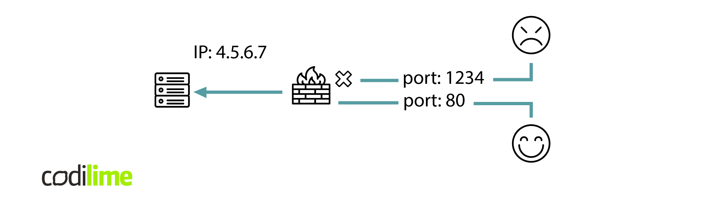
A firewall is an important component in protecting a network from attacks. It allows configuration of what kind of traffic is allowed inside the network. So in a sense, a firewall is a barrier that can reject all suspicious connections at the very entrance to the network, making potential attacks significantly more difficult.

There are many types of firewalls. In this article, we will focus only on simple stateless firewalls that work in the 3rd and 4th layer of the OSI model (L3 + L4 firewalls).

How to configure L3 + L4 firewall rules

Typically, a firewall uses a user-specified access control list (ACL) to decide which packets to let through and which to block.

An ACL is a list of rules along with associated actions. Each rule has a number of fields that specify the value ranges of packet fragments. The most common is a set of five fields – protocol (any or a specific one, such as UDP), source and destination IP (defined by prefix and mask pair), and source and destination port (defined as arbitrary ranges).

The main idea of processing such lists is straightforward – an incoming packet is compared with successive rules from the list. We find the first rule that matches the incoming packet and then perform its assigned action.

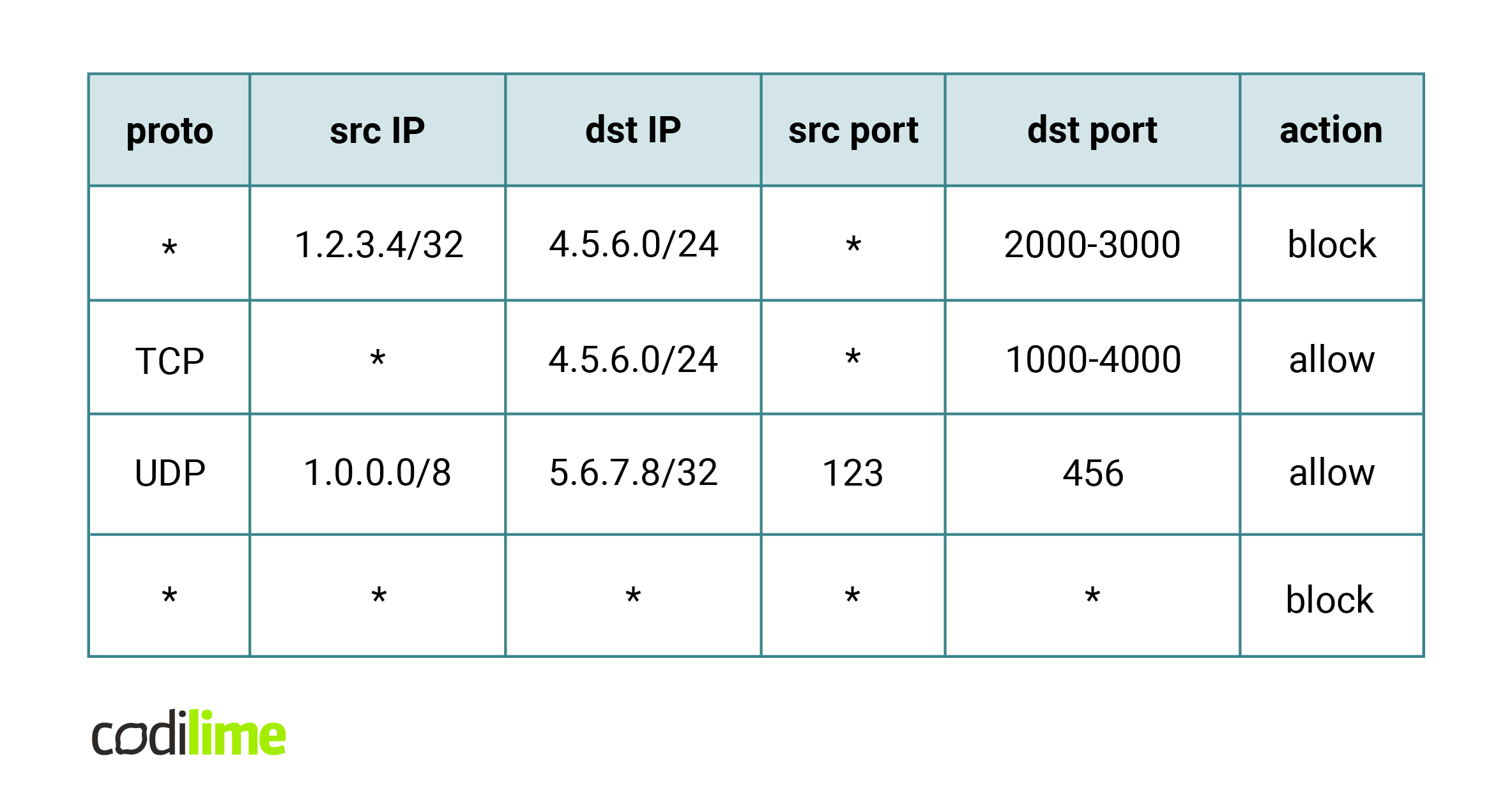
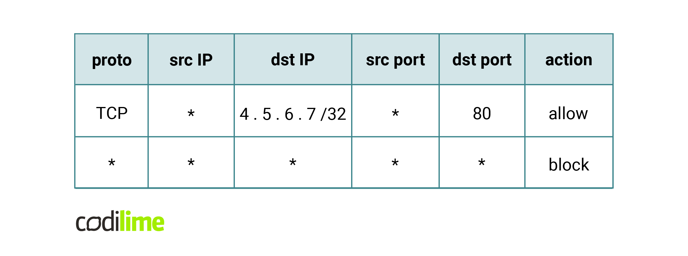
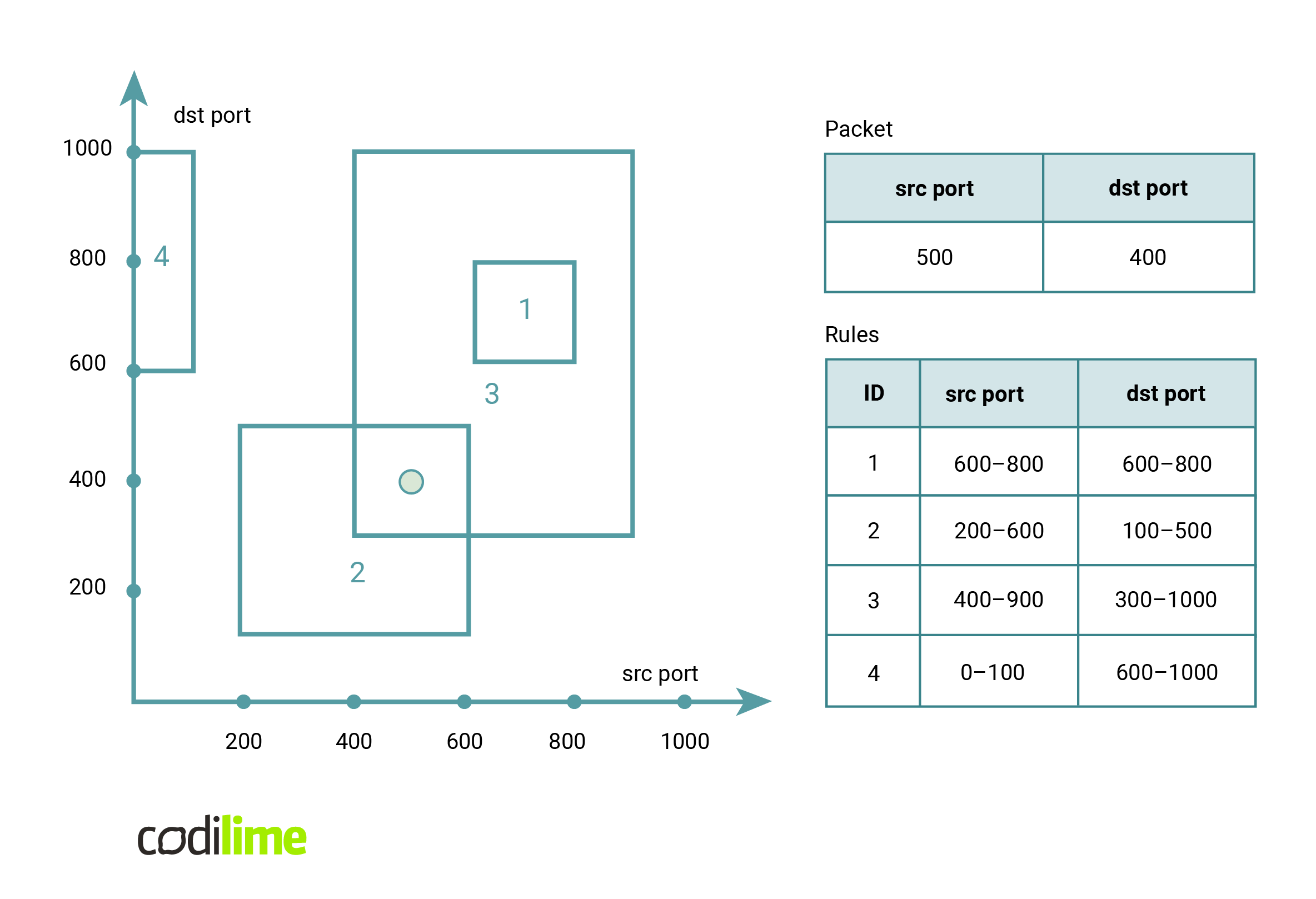
One can easily configure the firewall in the first figure with the following ACL:

Where else can you find uses for ACL? In fact, anywhere we want to manage network traffic. Also, nothing stands in the way of managing the list of rules automatically. This allows using an ACL to manage traffic in software-defined networking (SDN), or to block DDoS attacks. In these cases, it’s crucial to manage large rule sets efficiently.

These use cases impose some constraints on algorithms that process ACLs:

• support for a large number of rules (up to 10,000),
• quick response to queries about finding a matching rule for a given packet,
• fast rule set modifications.

With such requirements, one can start thinking about potential solutions.

Is there an optimal algorithm for an ACL?

The simplest algorithm for ACL processing iterates over successive elements of the list and finds the first rule that matches the given packet. It's worth considering whether such an algorithm is fast enough.

Let's assume that we want to process 10 MPPS (mega packets per second) and we have 1,000 rules. In such a situation, in the most pessimistic case, each packet will match the last rule. This means that to process 10M packets, we will need 10^10 checks. This can be achieved, but it will require a lot of computing power. Besides, we can often encounter traffic much larger than 10 MPPS, which would require even more computational power. So we see that the search for a better algorithm is definitely justified.

Let's look at the packet processing problem from a different angle. Each rule defines some consistent range of values on the five fields of the rule. Querying a packet, on the other hand, corresponds to finding a rule for which the corresponding parts of the packet lie inside the corresponding intervals of the rule. If we wanted to represent this graphically, rules would be hyperrectangles in a five-dimensional space, while a packet would be a point in that space. A query to find a rule for a given packet would correspond to finding the hyperrectangle with the smallest identifier that contains the point. Since it is hard for a human to imagine five dimensions, here is an example limiting ourselves to two dimensions.

It turns out that this problem is similar to several known geometry problems:

• Orthogonal Point Location: Given n non-intersecting rectangles, the query asks in which rectangle the given point lies.
• Orthogonal Point Enclosure Query: Given n arbitrary rectangles, the query asks for a list of all rectangles that contain the given point.

These problems are well studied and there are no algorithms that can perform operations in 5D faster than O(log^3 n) while maintaining a reasonable amount of memory consumption. As the packet classification problem is quite similar to these problems, we can suspect that there is no algorithm that can perform queries faster than O(log^3 n). In such a case, when the number of rules n = 1024 the query would take at least log^3 n = 1000 operations, so we haven't gained much.

Practical algorithms for ACL

We have shown that the optimal solution to the general problem is not easy. So is there any hope for a better algorithm?

Instead of looking for an algorithm that works fast in general, let's try to find an algorithm that works well in the world of computer networks. Let's consider whether we can make any assumptions about the rule set.

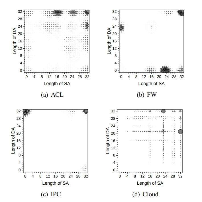
Take, for example, a DDoS attack. What would rules blocking such an attack look like? There would be a lot of rules blocking narrow ranges of source IP addresses. It's also easy to imagine that in other cases, there might be a lot of rules that have a specific destination IP address set, but the source IP is arbitrary.

In contrast, rules that span a large range of source addresses and a large range of destination addresses are relatively rare. Thus, we see that certain types of rules are significantly more frequent than others. It turns out that in a typical rule set, the number of different pairs (source mask length, destination mask length) is much smaller than the number of all such pairs.

Fig.6: The distribution of pairs (source IP mask length, destination IP mask length) in different rule sets. Each dot corresponds to a pair of mask lengths. The size of the dots corresponds to the number of rules with the same pair. ACL, FW, IPC, and Cloud are names of different rule sets.Source: https://arxiv.org/pdf/1909.07159.pdf      

So we can try to create an algorithm based on this observation. Its complexity would depend on the number of different pairs of address lengths.

Tuple Space Search

Tuple Space Search (TSS) is an algorithm for packet classification used in Open vSwitch       (OVS). The paper that describes TSS can be found here      .

Before diving into the algorithm, I will introduce the notation that will be used for the rest of the blog post. Assume we have an IP address range, for example, 1.2.3.0/24. Let's write it in a binary form: 00000001.00000010.00000011.00000000/24. The part that corresponds to the network (which is 000000010000001000000011 after omitting the dots) is called a prefix. The 24, which is the length of the subnet mask, is called the mask length.

Also, we will use an alternate way to write this kind of address range – we will write it as 000000010000001000000011******** which means any address that starts with 00000001.00000010.00000011 and ends with 8 bits representing the host part of the address.

We will also assume for a moment that the port ranges are given in a similar form as the IP address ranges. For example, the range [80; 95] can be represented as *000000000101****(because 1010000 is equal to 80 in binary and 01011111 is equal to 95). This obviously limits the possible sets of ports but will simplify the algorithm. In a later section, I will show how to deal with this limitation.

Notice that we can use this representation for the protocol field too. A protocol is either arbitrary (which corresponds to ******** in our notation) or is set to a specific value (like 00010001 = 17, which is UDP). So the mask length is either 0 or 8. That means we can use this notation for all five fields of the rule.

This notation will allow us to show examples with an arbitrary number of bits. Instead of writing 32 characters every time an IP address appears, which would be hard to read, we will use shorter addresses. For example, 1001** would mean 6-bit addresses with a prefix equal to 1001 and two arbitrary bits at the end.

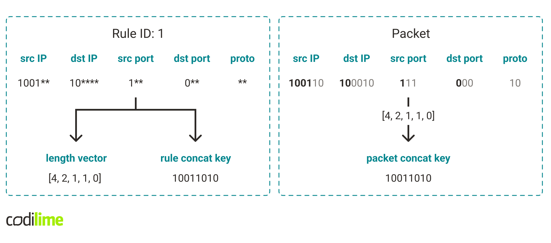
Based on this notation we can introduce the following definitions:

• Rule length vector – a five-element list containing all rule mask lengths.
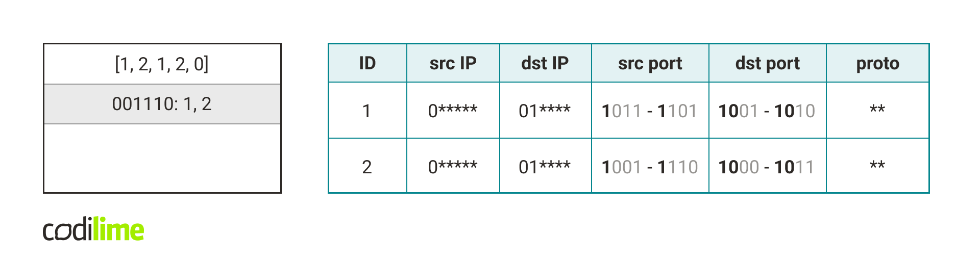
• Rule concat key – a concatenation of the field prefixes into a single value.
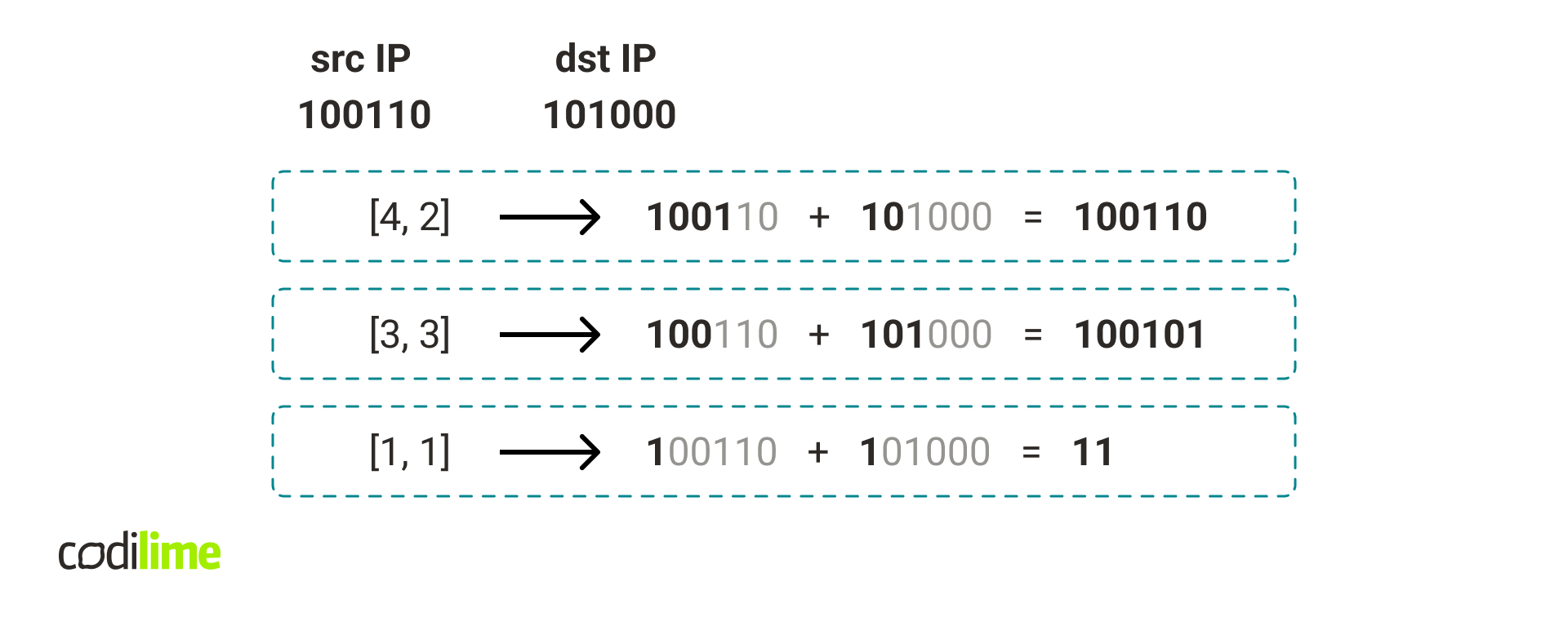
• Packet concat key for a given length vector – a concatenation of the packet fragments (in binary form) corresponding to the given length vector into a single value.

Take a look at Fig. 7. for an example.

How can we check if a rule matches a packet? One can think of it in such a way that we check the fields of a rule one by one. If a rule field has a mask length n, we compare the prefix of that field with the first n bits of the corresponding packet fragment. It turns out that this can be easily expressed using concat keys. Just check that the rule concat key is equal to the packet concat key for the rule's length vector.

If we assume that all rules have the same length vector, then the classification problem would come down to finding a rule whose concat key is equal to the concat key of the packet. This can be easily done using a simple hash table      .

But what if we have rules with many different length vectors? We can group rules by their length vector, create a hash table for each group and check each one when querying.

Adding a new rule

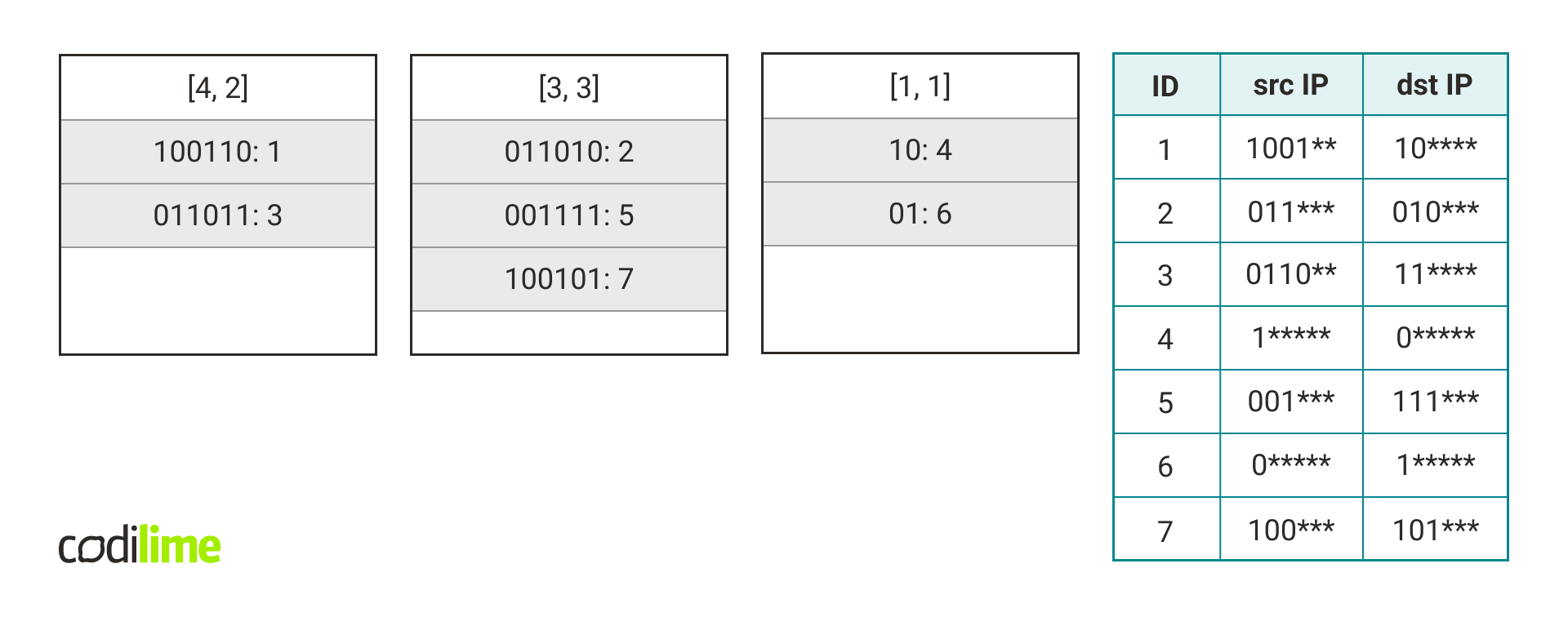
Each length vector is assigned to one hash table. For a vector of length L, let's denote such a hash table by hashtable(L). When a new rule R appears, the pair of length vector and concatenated key (L, K) is computed for it and we add rule R under key K to hashtable(L).

For the sake of simplicity, I will assume that the rules consist of IP addresses only. Generalizing the algorithm for all rule fields is trivial.

The following figure shows the contents of the hash tables after adding all the rules from the table.

Query Handling

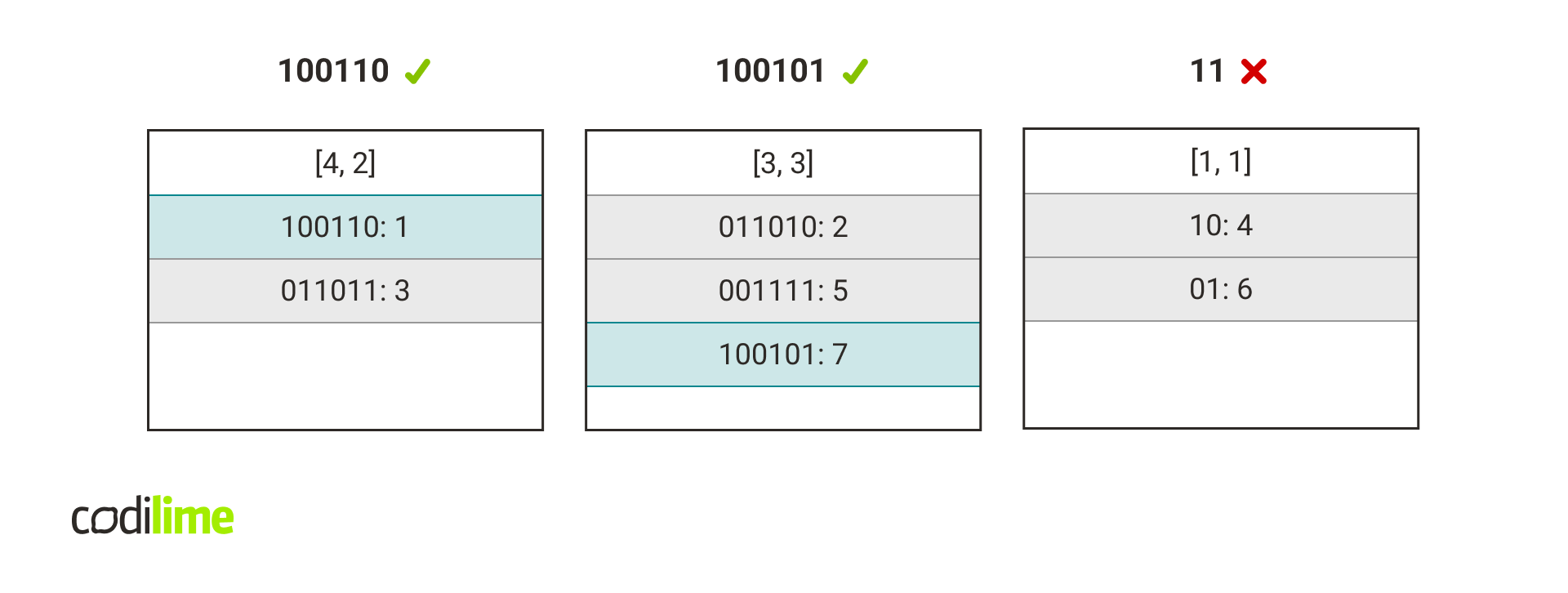
To classify a packet we first calculate the packet concat key for each existing hash table in our data structure.

Next, we check if the packet concat key occurs in the corresponding hash tables.

What to do with the port ranges?

Earlier I assumed that port ranges are represented by a notation with a prefix and *. However, we cannot assume this in practice. How to deal with this? The most common solution is to simply replace any port range with a larger port range that can be expressed in our notation. Below is an example.

This solution is very simple but has some drawbacks.

First, it generates false positives when handling queries – a packet may contain a port that did not belong to the original port range, but matched the rule after the port range expansion. The solution to this problem is to simply check that the rule we read from the hash table actually matches the packet.

The second problem is that several different rules can have the same key in the hash table. This can be solved by keeping lists of rules with the same hash. Then, at query time, we check all the rules in the list. This, of course, is a significant drawback to this solution but in a typical use case the number of such collisions should be small.

Tuple Space Search summary

Tuple Space Search is an algorithm that depends mainly on the number of different length vectors. Even though theoretically the number of length vectors can be as high as around 300K, in practice the number is much smaller. This shows how much we can gain by not operating on a completely arbitrary data set, but on data that is common in computer networks.

TupleMerge

TupleMerge (TM) is an algorithm used in Vector Packet Processing (VPP). It’s an extension of Tuple Space Search. The paper that describes TM can be found here      .

TupleMerge tries to reduce the number of hash tables in Tuple Space Search by merging several hash tables into one.

Hash tables merge

In Tuple Space Search, many similar rules are added to different hash tables because they differ slightly in length vector. This in turn increases the number of operations needed to handle a query. Maybe we could reduce the number of hash tables by “merging” some of them into one?

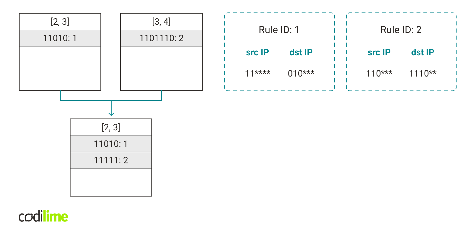
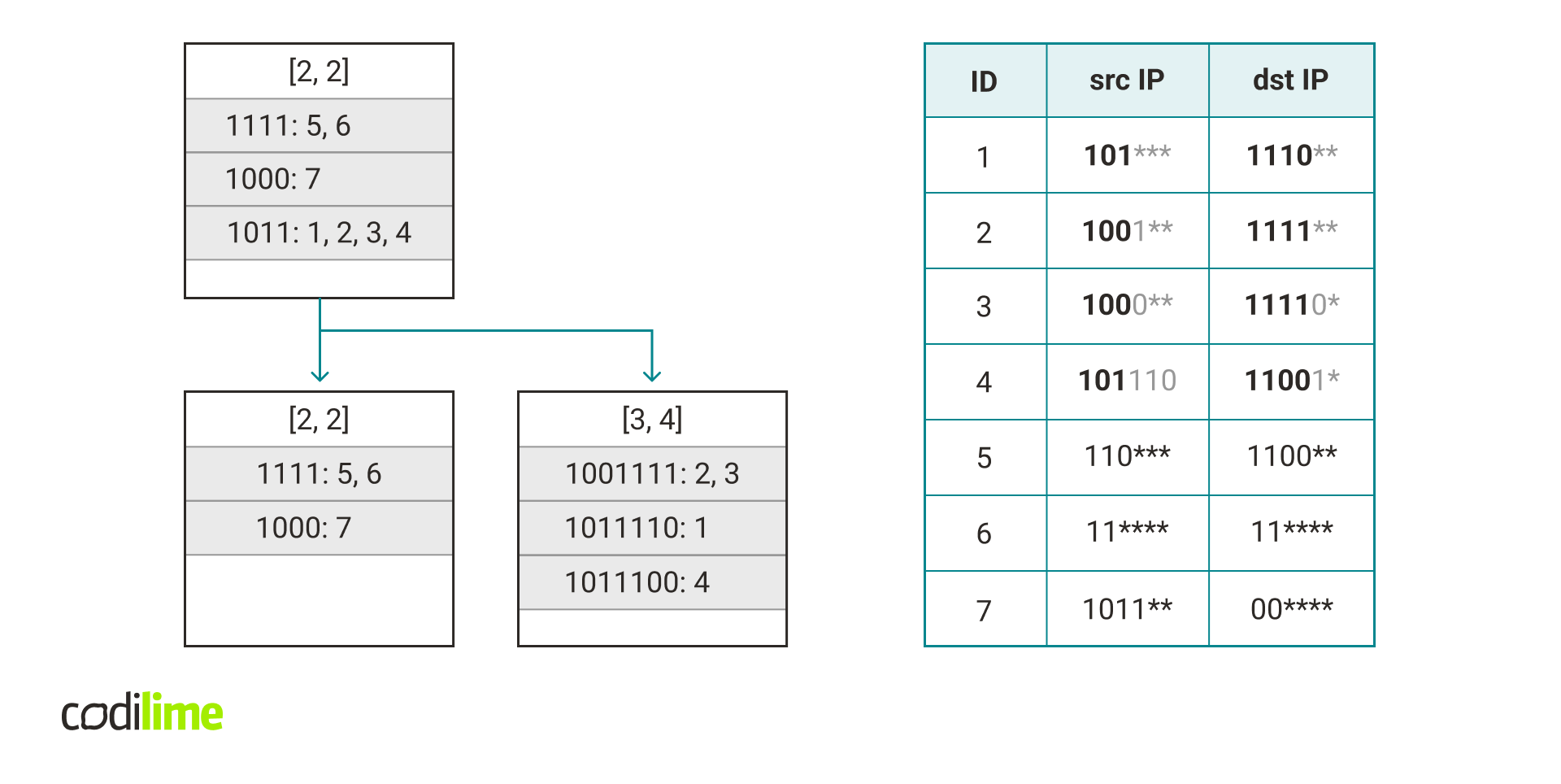
The main idea is to take a rule that is more specific and, by ignoring some of the bits, add it to a hash table containing less specific rules. For example, if we have a rule that has a length vector [3, 4], we can change the last bits from each field into * and get a rule that has a length vector [2, 3]. It would allow us to add this rule to other rules with length vectors [2, 3].

Merging reduces the number of hash tables at the cost of an increased number of false positives and collisions. But if we do it right we can greatly reduce the number of hash tables and accelerate packet classification by a large factor.

Choosing a hash table for new rules

In Tuple Space Search we always add a rule with the length vector L to the hashtable(L). In TupleMerge we will relax this requirement a little. We want to avoid creating new hash tables because it slows the queries down. But sometimes creating a hash table is unavoidable. In this case, we want to create such a hash table that would allow us to store the new rule with similarly structured rules that will appear later.

Notice that when we have a rule with length vector [a1, a2, …, an] then we can add it to a hash table with length vector [b1, b2, …, bn] if for each i: bi ≤ ai. In this case, we say that the rule is compatible with the hash table.

Let’s say we are adding a rule r with a length vector [sip,dip,sport,dport,proto]

• If there exists a hash table h that is compatible with r, we can just add r to h.

• Otherwise, we need to create a new hash table. Of course, we want to store r in it, but also want it to be compatible with other similar rules that will appear in the future. To achieve this, instead of using the length vector of r to create the new hash table, we could modify this vector a little by decreasing some fields.

  • If sip - dip > 4, set dip = dport = 0. Intuitively it checks whether the rule is more related to the source compared to the destination. If so, it ignores the destination, which allows storing other rules that are more related to the source in the same hash table.
  • If dip - sip > 4, set sip = sport = 0.
  • Set sip = sip - ⌊sip / 8⌋ (⌊x⌋ means taking the greatest integer less than or equal to x).  Intuitively it allows for adding rules that are slightly less specific to the same hash table.
  • Set dip = dip - ⌊dip / 8⌋.

Coping with a large number of collisions

Merging multiple hash tables can lead to a greater number of collisions. When adding a new rule, we can check how many rules there are in the hash table under the same key and if this number is too high, we can take some action to reduce the number of collisions.

Let’s denote C = maximum number of collisions.

Assume after adding a rule there is a list with more than C rules. In that case, we want to take these rules and move them to another hash table (the algorithm moves all of these rules to one specific hash table). How to choose this new hash table? We want to minimize the possible number of collisions so we will add these rules to the hash table with the maximum possible length vector that is compatible with all of these rules (i.e. the most specific hash table that can store all of these rules). This vector can be calculated by taking the minimum of the mask length for each field in this set of rules.

It’s possible that we are unlucky and all of these rules are added under the same key again. In this case, we should choose another way to split these rules. We can accomplish this by choosing a length vector such that only some rules from the list can be moved to the hash table with this vector.

Summary

The packet classification problem is an important component of computer networking so solving it as optimally as possible is crucial. In this blog post, we argued that this problem cannot be solved quickly in general, but there are heuristics that can solve it optimally in a typical use case.

In computer science, there are often problems that cannot be solved efficiently. In such situations, it is worth considering whether perhaps we can add some assumptions (that are true in a typical case) that will allow us to speed the algorithm up. Then such an algorithm, instead of always running slow, will slow down only in very specific situations that may actually never happen.