


In this blog post, we would like to address the topic of time series classification. This continues our consideration of the practical use of time series in the domain of networks and cloud infrastructure. In this article we focus on a use case related to distinguishing resource consumption characteristics (e.g. CPU, memory) for different workloads in a computing cluster. We describe in detail an example time series classification pipeline based on time series imaging and a convolutional neural network classifier.
Time series classification and why should you care
The term "time series analysis" encompasses various techniques, ranging from forecasting and seasonal pattern recognition to periodicity analysis, trend analysis, correlation, and causality analysis. Time series classification is also part of this spectrum. In a broader sense, classification is a supervised learning task (see our blog post about AI and Machine Learning for Networks: classification, clustering and anomaly detection) involving assigning observations to one of a number of predefined classes. How does this work in practice in the context of time series? To illustrate, let us consider the following example.
In sports analytics, particularly within running disciplines, accelerometer data collected over time from wearable devices worn by athletes can be used to classify various running styles such as "regular running," "sprinting," "jogging," "hill running," or "interval training," either through athlete annotations or predefined criteria. Athletes and coaches can leverage the classification results to gain insights into running performance, identify areas for improvement, and optimize training strategies to enhance overall athletic performance and prevent injuries.
Following the same paradigm, but this time for the IT domain, we will illustrate how to develop a classification model to distinguish between workloads in a computing cluster, specifically targeting time characteristics of resource consumption (memory/CPU) over time. Our objective is to identify workloads exhibiting daily patterns with distinct peak and off-peak periods. This knowledge can improve the efficiency of workload scheduling, e.g. by making a decision to place workloads having mutually shifted peak and off-peak on the same cluster nodes or scheduling time-limited workloads (such as job pods) during recognized off-peak periods. (For further insights, refer to our webinar on AI-powered scheduling in Kubernetes ![]() ).
).
Spectrograms as feature representations of a time series
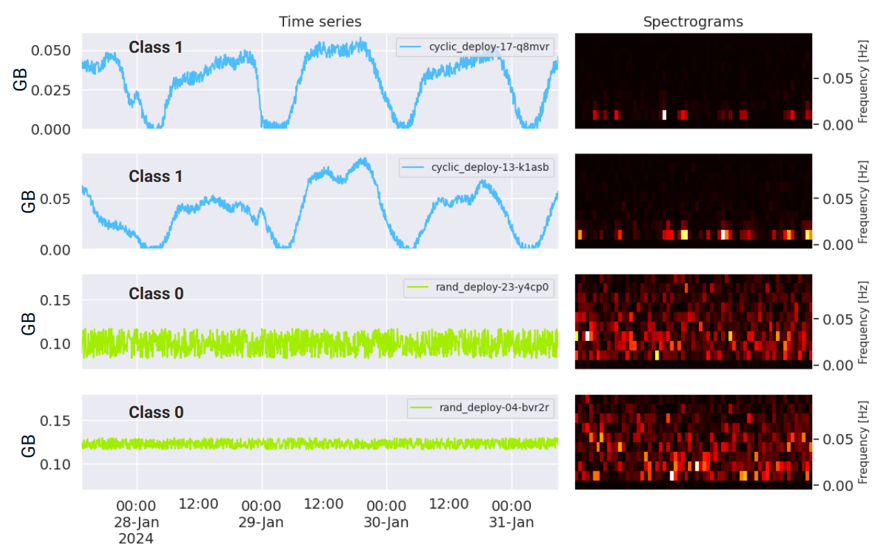
Examples of four characteristics for resource consumption (e.g. memory) are shown in Figure 1. The first two graphs in Figure 1 are representative of class 1, while the next two are class 0. A definite difference between these characteristics is evident. Memory characteristics for the first two pods presents a clear cyclicity, which is absent for the last two pods.
The classification problem within tabular data, where each observation is characterized by a set of features, is widely acknowledged in the realm of machine learning. Over time, numerous algorithms have been devised to address this challenge. Among the notable examples are decision trees, logistic regression, artificial neural networks, and support vector machines (SVM).
Time series data differs from other data types due to the significance of the sequential order of observations over time. Consequently, employing algorithms specifically designed for tabular data classification might not be straightforward. It necessitates the transformation of time series data into a comprehensive set of tabular features. In machine learning, features characterize and distinguish individual observations. In our case, a single observation is a time series. Examples of the simplest features extracted from raw time series data include mean, median, standard deviation, maximum value, and minimum value. In such a representation, each row denotes a distinct time series, with consecutive columns housing values derived from different features extracted from the raw time series data. A notable Python package that aids in this process is tsfresh ![]() , which is proficient in computing a wide array of diverse features. However, adopting this approach would entail intricate and labor-intensive feature engineering analysis to develop an effective classifier.
, which is proficient in computing a wide array of diverse features. However, adopting this approach would entail intricate and labor-intensive feature engineering analysis to develop an effective classifier.
This prompts the question of whether there is a simpler way to transform time series data into a format compatible with existing classifiers. One solution we have explored is representing time series as images, specifically using spectrograms. By doing so, we can leverage convolutional neural networks (CNNs), which are well-suited for image classification tasks, to analyze the data. A CNN is a type of deep learning algorithm commonly used for analyzing visual data, like images. It consists of multiple layers of convolutional filters and pooling layers that automatically learn hierarchical representations of features from raw pixel data, making it highly effective for tasks like image recognition and classification.
A spectrogram is a graphical representation of a time series in the time-frequency domain, see the example in Figure 1. From a practical point of view, it allows you to easily distinguish signals that exhibit a cyclic character from those that do not - as also seen in Figure 1.
Distinguishing between the spectrograms for the two identified classes is straightforward. Spectrograms belonging to class 0 exhibit a notably higher number of components compared to those of class 1. This difference stems from the cyclic nature of the signals in class 1. As a result, we have legitimate grounds to expect that representing the time series through spectrograms will facilitate classification by a CNN model.
It is worth emphasizing that the size and resolution of the figure remain consistent for all time series, regardless of their lengths. It is very convenient and required for further processing. Larger and more detailed figures typically lead to higher classification accuracy, but they also demand greater computational resources during both training and inference phases. Therefore, it is advisable to keep the figures as compact as possible to minimize computational overhead while still achieving the desired level of classification accuracy.
CNN fundamentals
Designing the architecture of a CNN involves decisions about the number of layers, their types, sizes, and the mathematical operations applied to the output of each layer, known as activation functions. It requires some skills and the process is iterative and tightly connected to the training process of the CNN described later. We will discuss the CNN architecture designed for the purpose of our task in the next section. However, to understand it, it is necessary to have a fundamental knowledge of the types of CNN layers and activation functions and their respective roles.
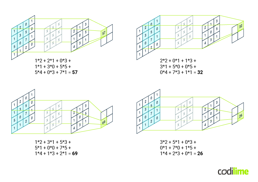
A convolutional layer serves as the core building block of a CNN. Figure 2 shows the idea behind the convolution, or in other words, cross-correlation. This process works like a sliding window over a grid of data, where a filter moves across the grid, multiplying its values with the corresponding parts of the data and adding them up as it goes. This helps to extract useful information from the data grid. By learning the appropriate filter weights during training, CNNs can automatically extract meaningful features from the input data, enabling them to perform tasks like image classification.
Figure 2 illustrates the process where a 3x3 kernel is slid across the input signal, which is initially of size 4x4. With each stride, the kernel traverses the input, performing the convolution operation. As a result, we obtain a feature map reduced in size from 4x4 to 2x2.
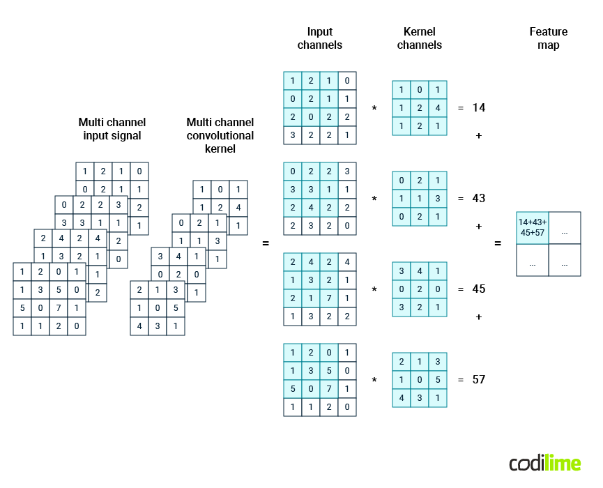
However, in a CNN, the input signal may consist of multiple channels as well. When a signal represents an image, each channel is a pixel matrix of a base color. Consequently, the convolutional kernel applied in such cases must also be multi-channel, with each channel having its own weight matrix. Figure 3 illustrates how the convolution process is carried out in such a scenario for a single kernel position (single stride). For each channel of the input signal, the corresponding channel of the kernel is subjected to element-wise multiplication and summation. The results for each channel are then aggregated. Consequently, at the end of this process, a single reduced matrix is obtained. A typical example of such an input signal is a multi-channel signal of a spectrogram image represented in 4-channel RGBA format.
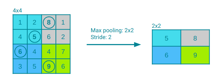
After the convolutional layers, pooling layers come into play to downsample the feature maps, effectively reducing their spatial dimensions while retaining essential information. In Figure 4, the pooling layer with a kernel size of 2x2 is depicted performing a maximum operation on the input layer, which condenses the output matrix dimension to 2x2. With a stride of two, the kernel shifts by two elements both horizontally and vertically while scanning the input layer. In pooling layers, aside from the max operation, other aggregating operations like average pooling, sum pooling, and several others can be used.
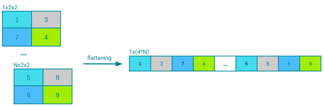
Following the convolutional or pooling layers, the flatten layer rearranges the output into a one-dimensional vector. This vector is then passed to the fully connected layers for classification. Figure 5 provides a visual demonstration of this process using a simple example.
Fully connected layers, also referred to as dense layers, establish connections between every neuron in one layer and every neuron in the subsequent layer. These layers play an important role in classification tasks by combining features learned from preceding layers, typically flattened into a one-dimensional input vector, and associating them with the output classes. While pixel values can constitute the input vector, it more commonly encompasses flattened feature maps derived from the image via convolutional layers.
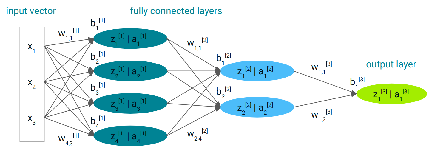
Figure 6 depicts a basic fully connected neural network, illustrating the weights and biases associated with each neuron and the values computed in each layer. In this network, each ith neuron in the first layer (denoted by [1]) computes its signal value $z_i^{[1]} = w_i^{[1]} x + b_i^{[1]}$, where $w_i^{[1]}$ represents the weights vector, $b_i^{[1]}$ denotes the bias and x is the input vector. Subsequently, it prepares the input $a_i^{[1]} = σ^{[1]}(z_i^{[1]})$ for the next layer, by applying the activation function $σ^{[1]}$ associated with layer 1 to the computed signal value.
Likewise, neurons in the second layer (denoted by [2]) compute their signal values $z_i^{[2]} = w_i^{[2]} a^{[1]} + b_i^{[2]}$, using the values produced by layer 1 $(a^{[1]})$ as input. The activation function $σ^{[2]}$ associated with layer 2 is then applied to the signal value, serving as the input for the subsequent layer.
Finally, the single neuron in the third layer (output layer, denoted by [3]) computes its signal value $z_i^{[3]} = w_i^{[3]} a^{[2]} + b_i^{[3]}$, utilizing the values produced by layer 2 $(a^{[2]})$ as input. It generates the final output $\widehat{y} = a_1^{[3]} = σ^{[3]}(z_1^{[3]})$ by applying its activation function $σ^{[3]}$.
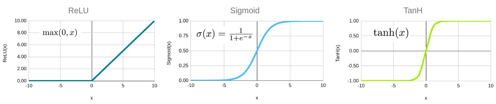
In a CNN architecture, an activation function plays a pivotal role by introducing non-linearity into the network, enabling it to capture intricate patterns and dependencies in the data. Applied to the output of each neuron, the activation function transforms the input signal into an output signal, which is then passed to the next layer. Figure 7 illustrates the widely used activation functions like rectified linear unit (ReLU ![]() ), sigmoid
), sigmoid ![]() , and hyperbolic tangent (TanH
, and hyperbolic tangent (TanH ![]() ).
).
The process described above is called forward propagation or forward pass. It involves processing of the input data, from the input layer through hidden layers to the output layer.
CNN design and model training
In order to train a model we need to have a training data set and structured CNN.
Data preparation
We started with a data set comprising time series data that represented CPU and memory consumption characteristics over time. These time series were labeled with either class 1 or class 0, denoting different patterns or behaviors. To enhance the diversity and robustness of our data set, we employed various data augmentation techniques. These techniques included generating new characteristics within specific classes, introducing different levels of noise, making local perturbations, and adjusting volume levels. By augmenting the data, we aimed to create a larger and more varied training data set, which improves the chances of developing a valuable classification model. Ultimately, our training data set consisted of 1000 time series labeled as class 1 and 2000 time series labeled as class 0. To prepare the data for training a CNN, we transformed the time series into spectrogram figures and their corresponding n-dimensional array representations.
Model construction
After experimenting with different configurations, we settled on the following architecture for our CNN.
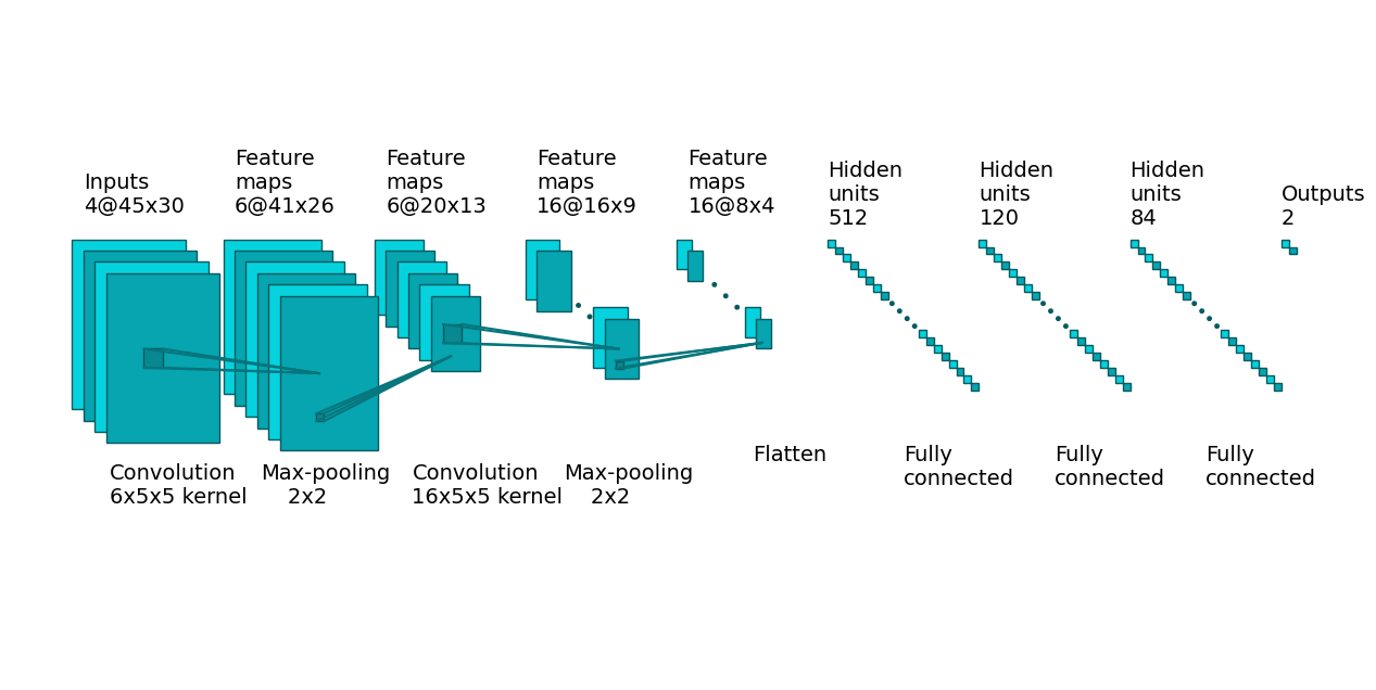
The initial convolutional layer in our architecture operates on a four-channel representation of a spectrogram image, i.e. three-channel RGB color model plus alpha channel. The input size of the spectrogram image is 45x30 pixels for each channel, resulting in an input matrix dimension of 4x45x30. This layer employs six kernels (filters) to compute feature maps. Each kernel has a weights matrix of size 4x5x5, which means that a separate 5x5 square matrix is applied to each channel in parallel (the computational mechanics here is similar as demonstrated in Figure 2 and Figure 3). As the 5x5 matrix is slid over each channel, the resulting feature map's size is reduced. Specifically, the position of the last 5x5 matrix on the 45x30 input channel is at coordinates 41x26. Therefore, after applying a single kernel (of size 4x5x5) we obtain a feature map of size 41x26 (as the summation over four input channels takes place at the end, see Figure 3 for comparison). However, the entire process is repeated six times, as we use six different kernels, as we mentioned. Since each kernel produces a distinct feature map, the layer generates a total of six feature maps, each measuring 41x26, for subsequent processing.
Following the convolutional layer, we transition to the pooling layer, where we employ the max pooling function for aggregation. This layer employs a square kernel of size 2x2 and a stride of two for sliding over input matrices, as visually depicted in Figure 4. After this layer, while the input data retains its six channels, the spatial dimensions of each channel are reduced from 41x26 to 20x13, as illustrated in Figure 8.
Next, we introduce the second convolutional layer, which operates on six input channels by utilizing 16 kernels of size 5x5. Post this layer, the data comprises 16 channels, each possessing a spatial size of 16x9, as observed from the reduction from 20x13 in Figure 8.
To further diminish the number of parameters requiring training, another pooling layer is employed with identical settings as the previous one. Although the data still contains 16 channels, the spatial dimensions are condensed to 8x4 from 16x9 - the output of the previous layer, as depicted in Figure 8.
The flatten layer (see Figure 5 for comparison), serves the purpose of converting the 16 feature maps, each sized 8x4, into a single 512-element vector. This vector is then fed as input into the fully connected segment of the network. These layers are crucial for classification tasks, utilizing the features extracted by the preceding convolutional layers.
In the fully connected part, the network takes the 512 features as input, followed by a layer that combines them into 120 features, and then another layer reduces them to 84 features, ultimately resulting in two numbers at the output of the third and final fully connected layer. The first number is a weight associated with class 1, the second one is for class 0, and the predicted class is determined based on which number is greater. Refer to Figure 8 for a visual representation.
As we mentioned before, designing CNN architectures is a complex task. It requires some skills and experience. The target CNN architecture we described above required experimenting with different configurations to achieve the satisfactory effect.
Model training
Initially, the weights and biases in a neural network are typically assigned random values. However, this random initialization does not guarantee accurate classification of input time series data. To improve the model's performance, the weights and biases must be adjusted iteratively during the training process using labeled training data. This adjustment involves selecting an appropriate optimizer and loss function.
In binary classification scenarios, a CNN is often configured to produce two values for each class, with the higher value dictating the final classification outcome. Through normalization, these values can be interpreted as the probability p of class 1 and 1−p the probability of class 0. In this context, binary cross entropy serves as the appropriate loss function:
$$\textit{Binary Cross Entropy} = -\frac{1}{N} \sum_{i=1}^{N} \left[ y_i \cdot \log(p_i) + (1 - y_i) \cdot \log(1 - p_i) \right]$$
N - is the number of samples in the data set
$y_i$ - is the true class label (0 or 1) of ith sample
$p_i$ - is the predicted probability that the ith sample belongs to class 1
To gain an intuitive understanding of binary cross entropy, consider this: if after processing a single time series belonging to class 1, we obtain an output p=0.9 (a good prediction), the loss function for that sample (assuming N=1) would be −log(0.9)=0.046. Conversely, if the output is p=0.2 (a weak prediction), then the loss function becomes −log(0.2)=0.799. This formula penalizes incorrect predictions, and typically, the loss function is evaluated across N samples (batch size, as explained later).
Loss functions serve as navigational guides for neural networks, aiding in the learning process by providing direction for adjusting model parameters to minimize errors. This adjustment process relies on gradients, which represent the rate of change of the loss function with respect to each parameter, offering valuable insights into the necessary adjustments to improve model performance.
Backward propagation, also referred to as backpropagation, is the mechanism by which gradients are calculated by traversing backward through the layers of the neural network. As information flows backward, each layer contributes to the overall loss, and backpropagation enables us to determine the degree of adjustment required for each layer to minimize this loss. By starting from the output layer and iteratively calculating gradients using the chain rule of calculus ![]() (enabling the calculation of the derivative of a composite function by sequentially applying the derivatives of its individual parts), the network can gradually refine its parameters, learning from its mistakes and improving its performance over time.
(enabling the calculation of the derivative of a composite function by sequentially applying the derivatives of its individual parts), the network can gradually refine its parameters, learning from its mistakes and improving its performance over time.
An example of an optimization algorithm ![]() commonly used in this process is the Adam
commonly used in this process is the Adam ![]() optimizer, which acts as an intelligent guide through the complex landscape of loss. By navigating through the highs and lows of the loss landscape, the Adam optimizer helps steer the training process towards more optimal parameter configurations. In our case, we opted for the default settings of the Adam optimizer, leveraging its proven effectiveness in practice to ensure reliable training of deep learning models.
optimizer, which acts as an intelligent guide through the complex landscape of loss. By navigating through the highs and lows of the loss landscape, the Adam optimizer helps steer the training process towards more optimal parameter configurations. In our case, we opted for the default settings of the Adam optimizer, leveraging its proven effectiveness in practice to ensure reliable training of deep learning models.
This iterative process of updating parameters based on computed gradients continues for multiple epochs until the model converges to a satisfactory solution. Each epoch involves multiple batches. An epoch refers to one complete traversal of the entire training data set through the neural network. On the other hand, a batch represents a subset of the training data set processed simultaneously in a single forward and backward pass of the network. Rather than processing the entire data set at once, it is segmented into smaller batches. These batches are processed sequentially, and following each batch, the network adjusts its parameters based on the calculated loss.
Model validation
To assess model performance, we partitioned the available data set into training (80%) and validation (20%) sets using a stratified split. This ensures that both sets maintain a similar distribution of class 0 and class 1 time series as seen in the original data set. Additionally, we selected a model evaluation metric.
The evaluation metric employed is the balanced accuracy metric, as defined and implemented in the scikit-learn ![]() Python package. This metric proves valuable, especially in scenarios featuring imbalanced classes, such as having 1000 out of 3000 time series belonging to class 1 and 2000 out of 3000 to class 0. The balanced accuracy calculates the average classification accuracy of each class, assigning equal importance to each class irrespective of its size.
Python package. This metric proves valuable, especially in scenarios featuring imbalanced classes, such as having 1000 out of 3000 time series belonging to class 1 and 2000 out of 3000 to class 0. The balanced accuracy calculates the average classification accuracy of each class, assigning equal importance to each class irrespective of its size.
For instance, if our model accurately classifies 60% of the time series from class 1 and 95% of those from class 0, the balanced accuracy is calculated as 0.5*(0.6 + 0.95) = 0.775, while the regular accuracy is computed as (1000/3000) * 0.6 + (2000/3000) * 0.95 = 0.83. In our case simply the balanced accuracy is a better metric than the regular accuracy.
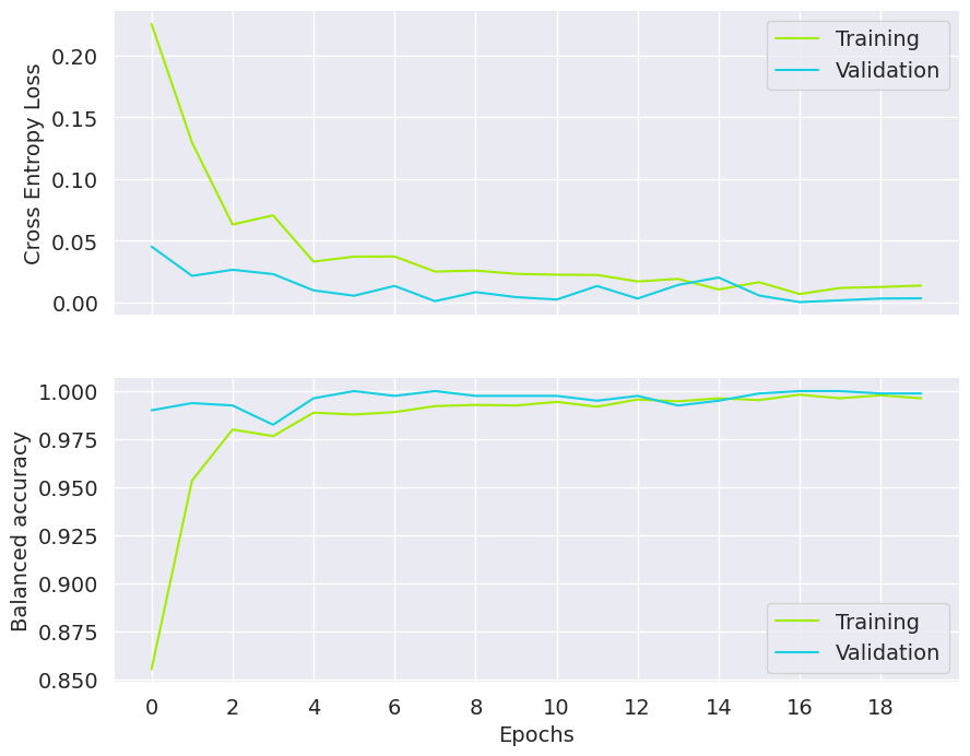
The model is separately evaluated after each training epoch for training and validation sets in terms of loss function and balanced accuracy (Figure 9). It is necessary for checking if the model is not overfitted (good results for training set and substantially worse for validation set - unseen during training) and for proper stop criterion (the next epochs are not necessary after achieving the required model performance metric). We see that the training loss decreases until the 16th epoch, and also the balanced accuracy for this epoch shows the best results. In the figure presented, the training should stop at the 16th epoch. In our classification task, the balanced accuracy is above 0.97 and is similar for training and validation sets.
Hyperparameters optimization
When working with CNNs, there are numerous parameters, known as hyperparameters, that are predetermined and not learned from the data itself. These parameters are crucial for optimizing the model's performance and are fine-tuned through a process of exploration and optimization. Among the most critical hyperparameters for CNNs are:
- Input data size: This parameter is closely tied to the size and resolution of the figures used during the transformation of raw time series data into spectrograms. It strongly influences the model training time and its final accuracy.
- Learning rate: This controls the step size during the optimization process, striking a balance between achieving accuracy and convergence speed.
- CNN architecture-related parameters: These include the number of convolutional layers, the number and sizes of filters within these layers, and the types and sizes of pooling layers employed, etc.
- Activation function: This function affects the model's ability to capture nonlinearities within the data.
- Batch size: This parameter influences the training process and the convergence behavior of the optimization algorithm.
- Optimizer: Along with its associated parameters, the choice of optimizer impacts the training dynamics and the final performance of the CNN model.
Systematically evaluating different combinations of these hyperparameters and selecting the best-performing configuration on the validation data is essential. Various techniques, such as grid and random search, Bayesian optimization, or evolutionary algorithms, can be employed for this purpose. However, it is important to note that this process can be computationally intensive, and experience plays a crucial role in narrowing down the hyperparameter search space effectively.
Inference pipeline
Once the model is trained, we can employ it for analyzing completely new data. Figure 10 illustrates the inference pipeline we have developed for time series classification using a CNN model.

When processing new input time series, it is crucial to follow the same steps used during the model training phase. This involves transforming the time series into a spectrogram figure using the same parameters as before: figure size, resolution, color schemes, and other relevant settings.
After this preprocessing step, the data is passed through the specific layers of the trained CNN model. Finally, the model outputs the class to which the input time series belongs.
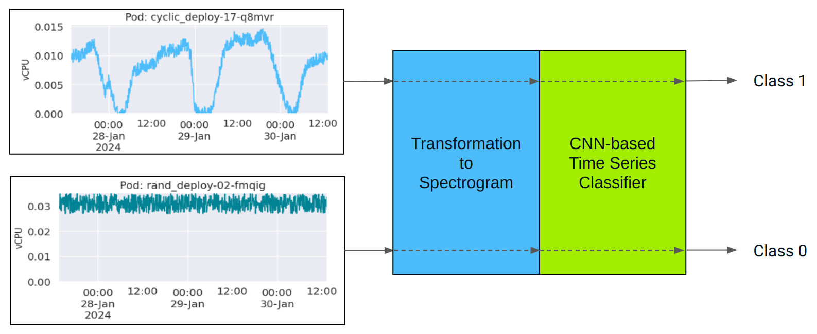
Figure 11 showcases the application of the trained CNN model for classifying time series data representing CPU usage of sample pods within a Kubernetes cluster. On the left side of the figure, two example workload instances are depicted. This visualization demonstrates the inference pipeline effectiveness in discerning between distinct workload classes based on their CPU usage characteristics.
Summary
Time series classification finds numerous applications in real-world scenarios, particularly in network and cloud environments where such data is prevalent. We have showcased an example of distinguishing between different workloads exhibiting distinct resource consumption patterns over time. This automated classification of workloads contributes to more efficient scheduling across computing cluster nodes. Our approach involved transforming time series into spectrogram figures, enabling the utilization of a CNN-based classifier. We have also outlined the advantages of this approach compared to traditional classifiers that operate on tabular, time series feature-based methods.


