Sentiment Analysis. What is it and how to use it?

During face-to-face conversations or by reading text - we, people, can determine a speaker's intention or mood, whether they feel happy about something or not. We can also identify the polarity of the context - is the expression positive or negative or maybe even neutral? 

It is relatively easy for most people, but do computers understand emotions? Is it important for machines to understand humans’ intentions? With the technological progression and advancement of machine learning techniques - our machines are getting closer and closer to answering these questions.

What is sentiment analysis?

Sentiment analysis is an NLP (Natural Language Processing) technique which helps detect the sentiment of a piece of text. Basically, this is the text’s classification - its polarity. These are algorithms that can quickly check large amounts of text and specify whether they have positive, neutral, or negative sentiment. Sentiment data analysis is also known as opinion mining. 

Why is sentiment analysis important?

Sentiment analysis is used by companies to determine opinions about a service or a product. A great example of this would be internet feedback forums or social media, where customers exchange their thoughts. Automating the process of verifying whether there’s positive or negative sentiment towards a product or service results in increased efficiency and makes it easier to make data-driven decisions. 

Learn more about big data on our blog.

Natural language processing and sentiment analysis are often used for analyzing the reviews posted on the internet. Companies are able to get useful feedback on product features, target audience or pricing. In addition, tracking the overall reviews and customers’ emotions might also be very useful for evaluating the success of marketing activities as well as identifying brand awareness.

Sentiment classification - positive and negative words

From natural language processing perspective, words can be categorized into three categories: positive, negative, or neutral. For example, positive and negative words will be scored with +1 and -1, and neutral with 0. The examples of words in each category are presented below.                             

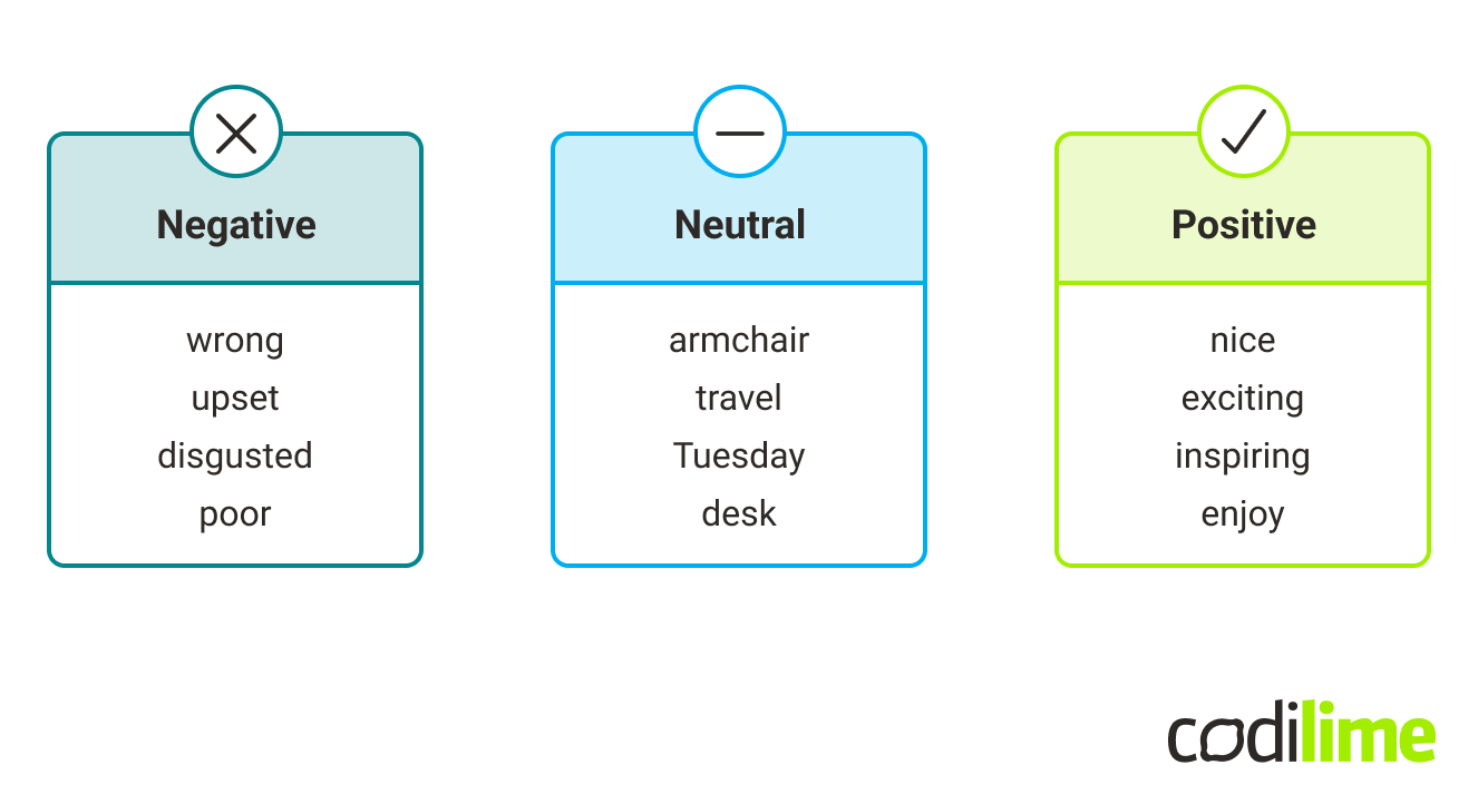
The sentiment analysis system categorizes key words of the sentence, and the summary of each word will give us an overall understanding of whether the sentence has a positive sentiment or a negative sentiment. 

To perform a simple analysis - let’s have a look at the example:

The movie was awesome!

STEP 1 

Remove unnecessary words and special characters from the sentence. Those unnecessary words are anything that does not add any meaning to the overall sentiment - such as the, me, a, are, is etc. Exclamation marks, question marks, commas, etc. - are the special characters which need to be removed as well, as they are not helping to determine the sentiment of the sentence. These are also called stop words. In the given example, that would be: 

The movie was awesome**!**

So we're only left with words:

movie awesome

STEP 2 

After cleaning the sentence, classify each word:

movie 0

awesome +1 

STEP 3 

The next step of sentiment analysis is to identify the polarity by summing up the scores of each word. Then we can conclude that the sentence has a positive sentiment. 

To determine the polarity of each word, the package TextBlob could be used as per below:

from textblob import TextBlob

print(TextBlob(“The movie was awesome!”).sentiment)

The output of the sentence has been clasified:

Sentiment(polarity=1.0, subjectivity=1.0)

The TextBlob library gives two outputs, as presented above. Polarity lies between [-1, 1], as we already discussed in this article. However, subjectivity lies between [0, 1], and refers to attitudes or personal opinions. 

Sentiment analysis model - how to do it?

With this short introduction, we can now perform sentiment analysis in Python on an existing set from Kaggle - Amazon Fine Food Reviews      . 

The dataset contains about 0,5 million reviews, including products - food from Amazon, user information, ratings (from 1 to 5) and the review itself.

The code for this exercise in sentiment analysis is presented in a notebook format in the author’s repository      .

Step 1: Libraries

Firstly, we will be importing the necessary libraries:

import pandas as pd #dataframe library

import numpy as np #linear algebra

import matplotlib.pyplot as plt #visualization

import seaborn as sns #visualization

plt.style.use('ggplot')

import nltk #natural language toolkit

Read and display the data:

df = pd.read_csv('Reviews.csv')

df.head()

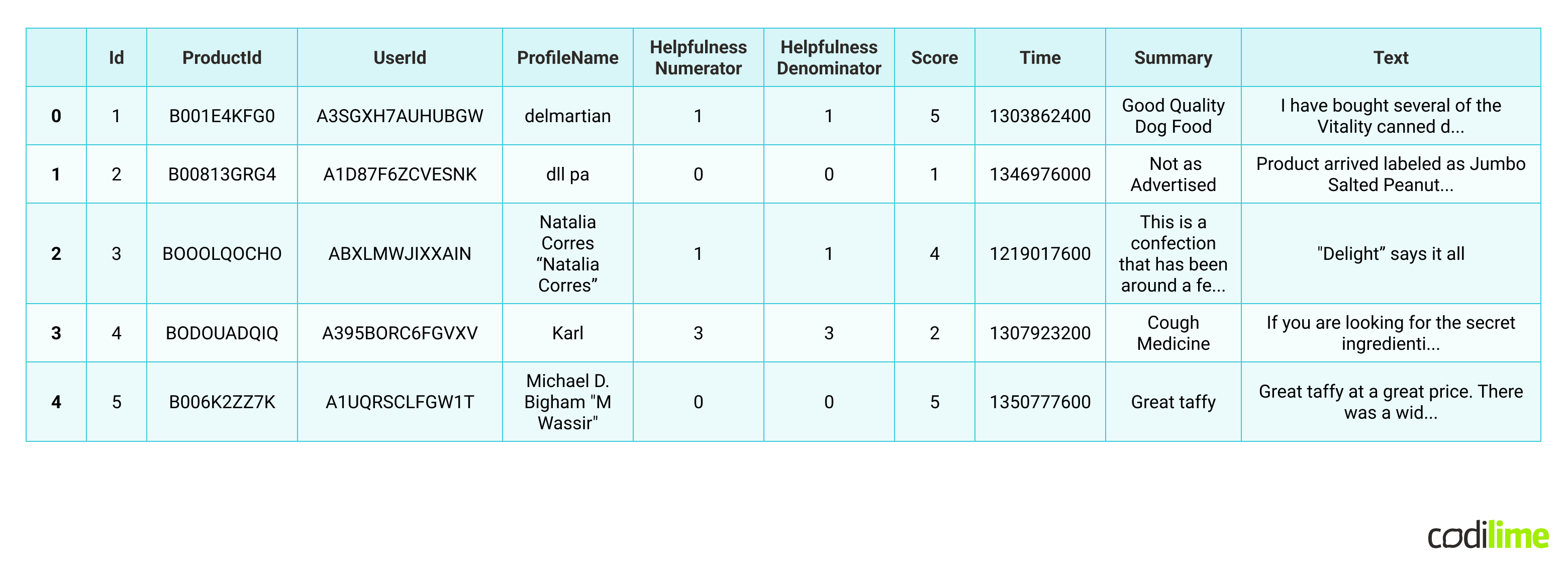
We can see following columns:

1. Id - unique id of each row
2. ProductId - an unique identifier for the product
3. UserId - an unique identifier for the user
4. ProfileName - profile name of the user
5. HelpfulnessNumerator - number of users who found the review helpful
6. HelpfulnessDenominator - number of used who indicated whether they found the review helpful or not
7. Score - food rating between 1 and 5
8. Time - review timestamp
9. Summary - brief summary of the review
10. Text - text of the review

The most interesting columns for us, to perform sentiment data analysis, are “Score”, “Text” and “Summary”. 

Step 2: EDA & NLTK

EDA gives you an idea of what the data looks like and how it is distributed. Let’s take a closer look at the “Score” column:

ax = df\['Score'].value_counts().sort_index().plot(kind='bar', title='Count of Reviews by Score', figsize=(10,5))

ax.set_xlabel('Review Score')

plt.show()

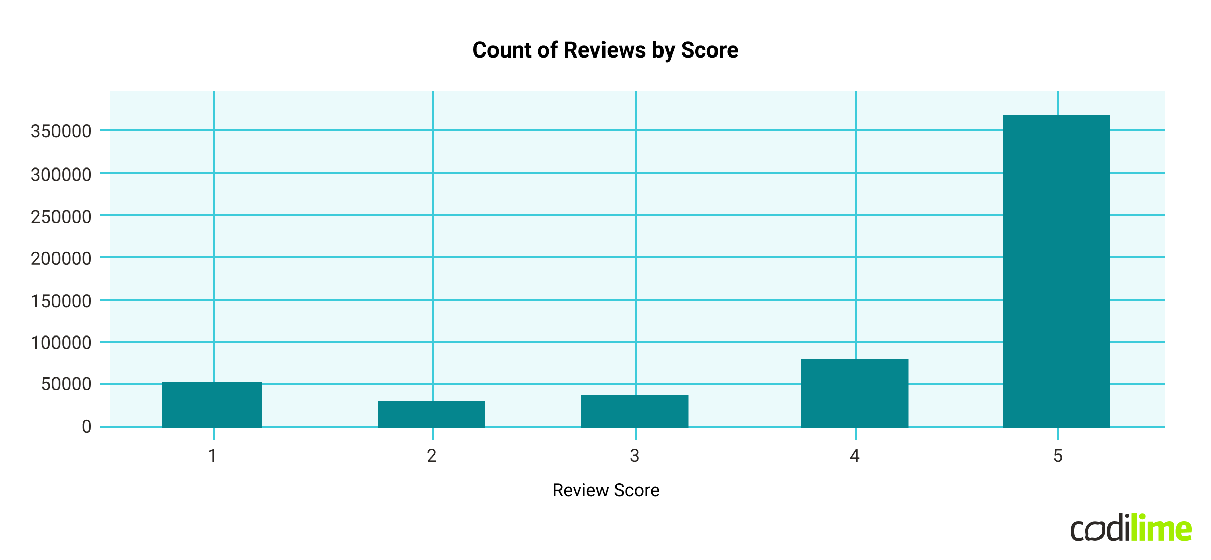
We can see that most of the reviews are 5 points. So that leads to the conclusion that our dataset is biased towards positive reviews.

Now let’s get more familiar with NLTK by performing some operations on an example review.

review_example = df\['Text']\[1000]

print(review_example)



“I never in my life tasted such a good babka its crazy good! This is the real babka! That my gram mother use to mak e”

The review seems to have a positive sentiment, but let’s split each word of the review into tokens. The NLTK package offers a function to tokenize the sentence, so let’s display the first 10. After performing that step, we will be using the part-of-speech tagging function, which refers to the categorizing of words in a text, depending on the definition of the word and its context. We will also display the first 10 tokens.

tokens = nltk.word_tokenize(review_example)

tokens\[:10]



tagged = nltk.pos_tag(tokens)

tagged\[:10]

In this article       you can find the meanings of each abbreviation.

For example:

PRP = Personal Pronoun. Examples: I, he, she 

JJ = Adjective

The next step of sentiment analysis would be putting these tags into entities. That takes the tagged tokens and groups them into chunks of text.

entities = nltk.chunk.ne_chunk(tagged)
entities.pprint()

Output:

(S

  I/PRP

  never/RB

  in/IN

  my/PRP$

  life/NN

  tasted/VBD

  such/PDT

  a/DT

  good/JJ

  babka/NN

  its/PRP$

  crazy/JJ

  good/JJ

  !/.

  This/DT

  is/VBZ

  the/DT

  real/JJ

  babka/NN

  !/.

  That/IN

  my/PRP$

  gram/NN

  mother/NN

  use/NN

  to/TO

  make/VB)

Step 3: Sentiment Classification Model 

After getting more familiar with the dataset and NLTK, we are now ready to build the model.

As input, the model will be taking the reviews. Then it will predict whether the review has a positive or a negative sentiment. In other words, we will classify the reviews - meaning this is a classification problem; hence we can start with one of the sentiment analysis algorithms - logistic regression. 

We are going to perform supervised learning. To do so, we will be adding an extra column which is going to classify the reviews into positive and negative - we will use it as training data for our sentiment analysis model. 

• Classification

That being said, we will classify all reviews with a score above 3 as +1 (positive sentiment). Below 3 as -1 (negative sentiment) and equal to 3 as 0 (neutral sentiment). We will remove the neutral reviews from our dataset.

df = df\[df['Score'] != 3]

df\['sentiment'] = df\['Score'].apply(lambda rating : +1 if rating > 3 else -1)

df.head()

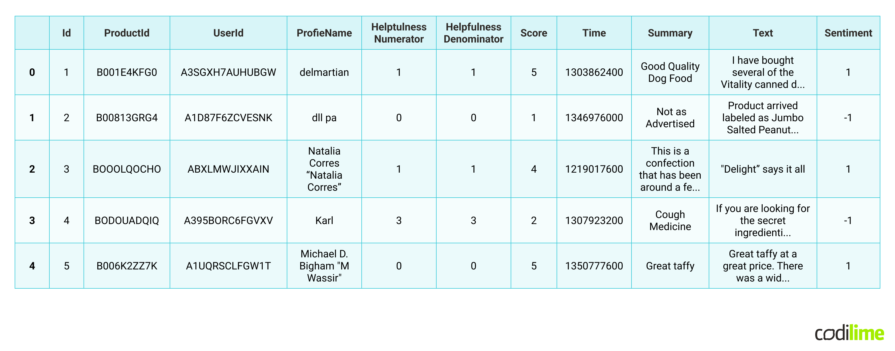
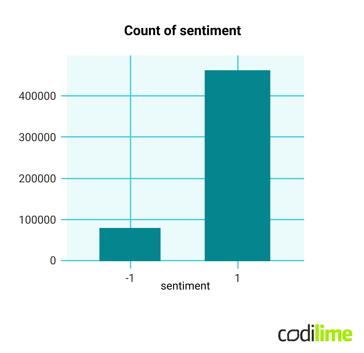
We can now again perform visualization to see the distribution after removing rows with neutral reviews.

ax = df\['sentiment'].value_counts().sort_index().plot(kind='bar', title='Count of sentiment', figsize=(10,5))

ax.set_xlabel('sentiment')

plt.show()

• Dataframe for the model & data cleaning 

We will perform some data cleaning by removing all punctuation (question marks, commas, etc.).

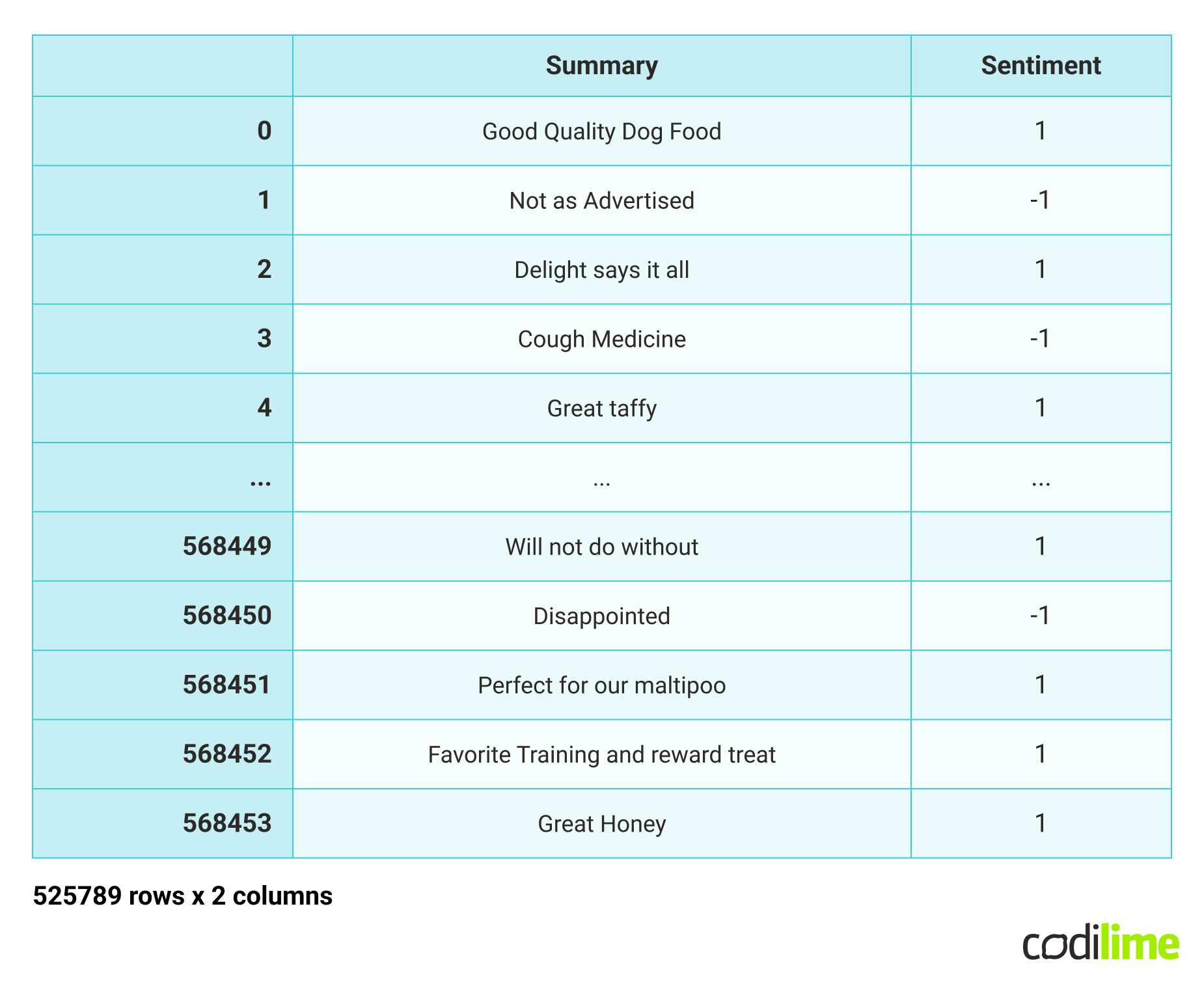
For our classification model, we will be using two columns: “summary” and “sentiment”. “Sentiment” is our target variable. 

def remove_punctuation(text):

    final = "".join(u for u in text if u not in ("?", ".", ";", ":",  "!",'"'))

    return final

df\['Text'] = df\['Text'].apply(remove_punctuation)

df = df.dropna(subset=\['Summary'])

df\['Summary'] = df\['Summary'].apply(remove_punctuation)



df_model = df\[["Summary", "sentiment"]]

df_model

• Split data into train and test sets.

We will perform a classic split: 80% of the data frame will be train data, and the remaining 20% we will use as a test set. To do that, we will be using the sklearn package. 

from sklearn.model_selection import train_test_split

X = df_model\['Summary']

y = df_model\['sentiment']

X_train, X_test, y_train, y_test = train_test_split(X, y, test_size=0.2, random_state=42)

Once we have split our data, it is almost time to train the model. However, there is one problem. The Logistic Regression algorithm does not understand text. To solve it, we would need to convert the text into a bag-of-words model. We can simply perform that using the sklearn package - CountVectorizer. CountVectorizer is used to transform a given test into a vector on the basis of the count of each word that occurs in the text.

from sklearn.feature_extraction.text import CountVectorizer

vectorizer = CountVectorizer(token_pattern=r'\b\w+\b')

\# vectorizer for splitted sets:

X_train = vectorizer.fit_transform(X_train)

X_test = vectorizer.transform(X_test)

• Logistic regression

After the preparation of our data, it is time to build the model, train the data on it and make predictions.

from sklearn.linear_model import LogisticRegression

lr = LogisticRegression()



lr.fit(X_train,y_train)

prediction = lr.predict(X_test)

• Testing & results

Let’s first have a look at the confusion matrix, which measures the performance of the model and presents a visual representation of the actual and predicted values.

from sklearn.metrics import confusion_matrix,classification_report

new = np.asarray(y_test)

confusion_matrix(prediction,y_test)

Output:

array([[10850, 2216],
      [5383, 86709]])

It already looks pretty good - looking at the number of TP (True Positive) and TN (True Negative) values. But let’s also run the classification report:

print(classification_report(prediction,y_test))

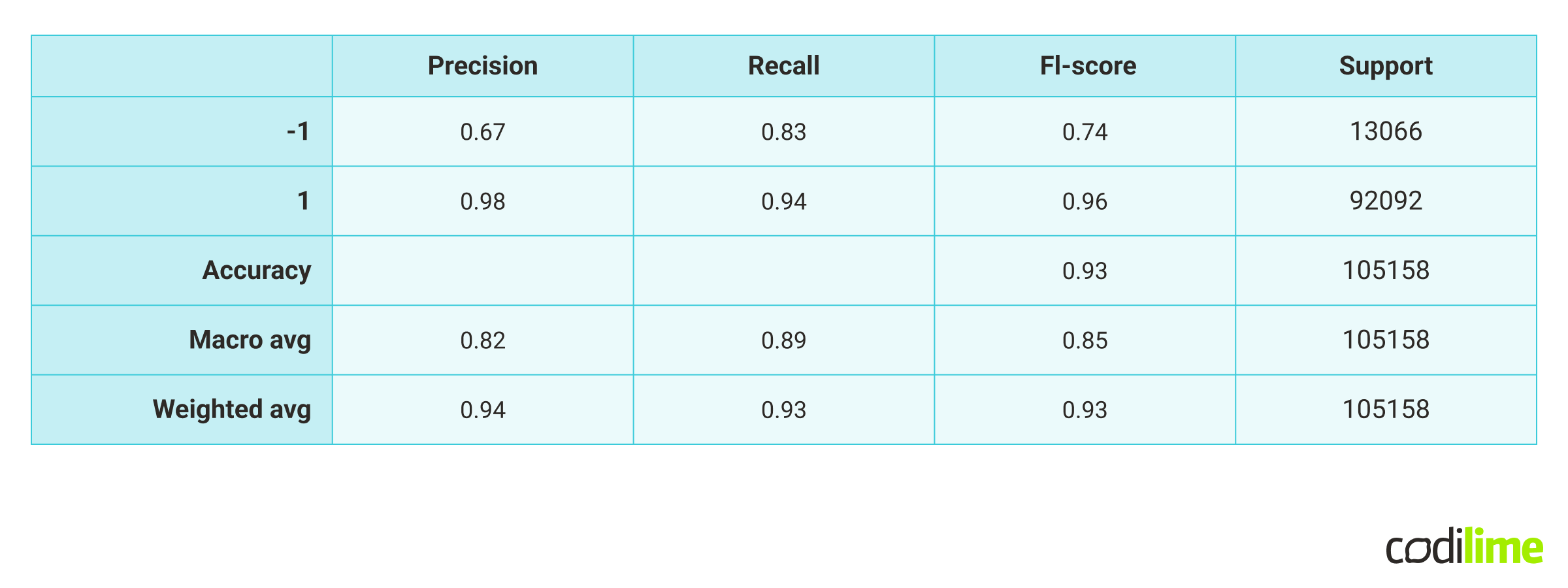
Looking at the report above, it seems like the model performs very well, with a satisfying, high accuracy. 

RoBERTa

We did classify the reviews with our model of natural language processing. But on top of that, I would like to introduce you to RoBERTa from Hugging Face. RoBERTa is a pretrained, more advanced transformer model for more accurate sentiment analysis systems. 

Human language depends a lot on context. Some reviews or sentences can sound negative, but might be just humorous and the sentiment overall could be positive. The model above is a simple logistic regression and it would not pick up those exceptions, the relationships between words. TextBlob, mentioned at the beginning of this article, also could not solve this problem.

RoBERTa is - as mentioned - an advanced, pretrained, transformer-based, deep learning model. The transformer model accounts for the words but also the context related to other words. You can read more about this sentiment analysis tool in the documentation      . 

Step 1

Let’s first import the necessary libraries, we will be importing AutoTokenizer, which will perform the same job as NLTK, but is also available in the transformer package. We will also need a model algorithm as well - AutoModel for classification. We will be using also using Softmax from SciPy, to apply to the final output:

from transformers import AutoTokenizer

from transformers import AutoModelForSequenceClassification

from scipy.special import Softmax

Step 2

We will be using a specific model, that has been pretrained on Twitter data - and based on that we will be doing transfer training:

MODEL = f”cardiffnlp/twitter-roberta-base-sentiment”

tokens = AutoTokenizer.from_pretrained(MODEL)

model = AutoModelForSequenceClassification.from_pretrained(MODEL)

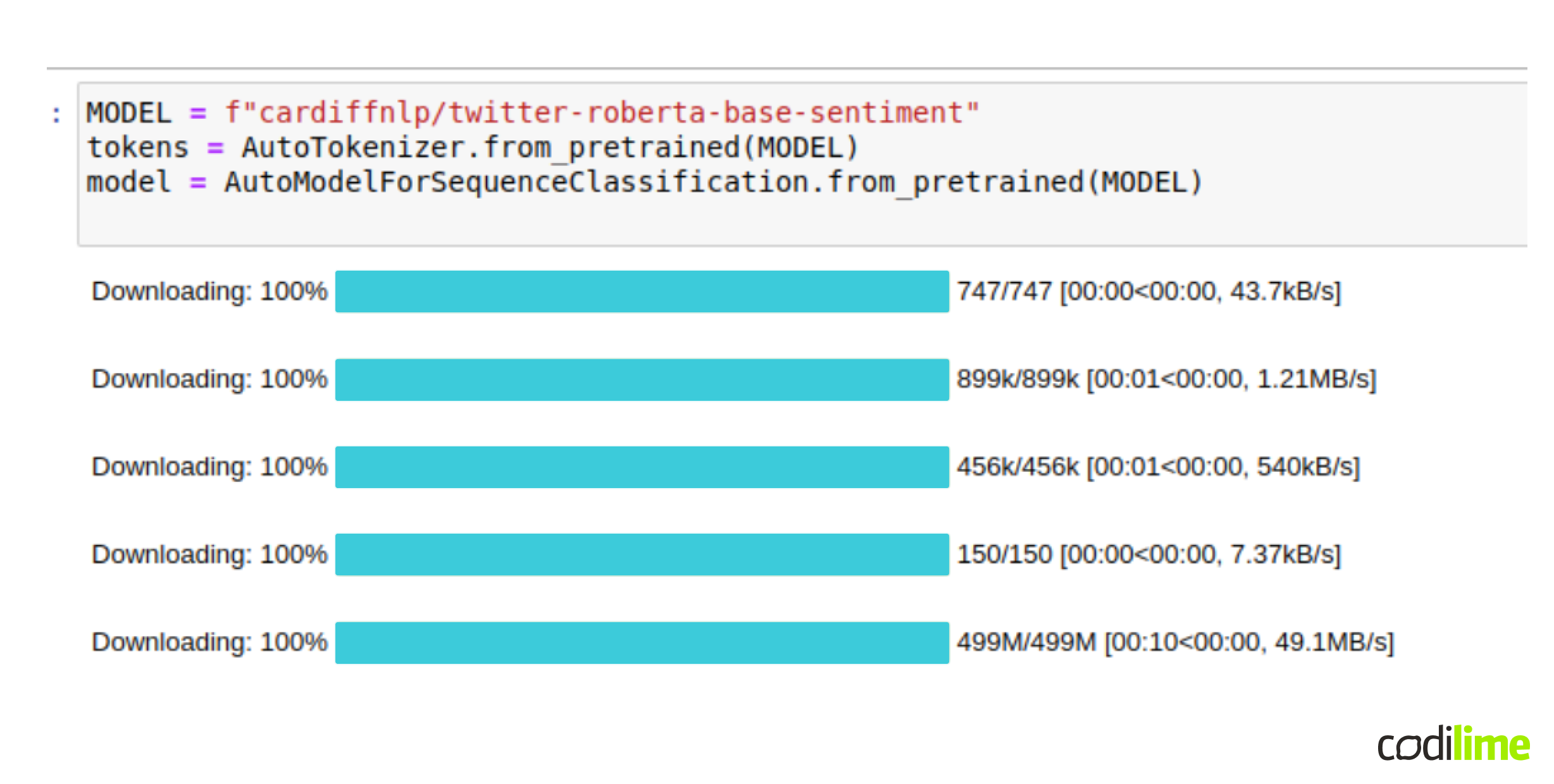
First, we need to download all of the weights - it might take some time, but that’s to be expected. After that we have a tokenizer and a model - we can easily apply it to our text now.

Step 3

Firstly, let’s encode the text by applying the tokenizer to our example review, already given earlier in the code: 

print(review_example)



“I never in my life tasted such a good babka,its crazy good! This is the real babka! That my gram mother use to mak e”

As per output, we got an encoded text, which the model will understand. And now we can simply apply the model. 

The output of this code is a tensor. We will be transforming it from the tensor form to numpy and store locally. 

The score would be as follow:

• Negative: 0.00378648, 
• Neutral: 0.02099775,
• Positive: 0.9752157

Which would make sense by looking at the example review. 

Let’s try to run this on the entire dataset. To do so, let’s create a function, which will take any given example review and perform everything we have written so far:

def roberta_scores(example_review):

    encoding = tokens(review_example, return_tensors ='pt') 

    results = model(\*\*encoding)

    score = results\[0]\[0].detach().numpy()

    score = softmax(score)

    dict_scores = {

        'negative' : score\[0],

        'neutral' : score\[1],

        'positive' : score\[2],

        

    }

    return dict_scores

And we can go through all the rows and apply our function:

from tqdm.notebook import tqdm

final_results = {}

for i, row in tqdm(df.iterrows(), total = len(df)):

    review = row\['Text']

    review_id = row\['Id']

    results = roberta_scores(review)

    final_results\[review_id] = results

Please note, it might take awhile, as it is iterating through 0.5 million rows! 

Anyway, we can now simply merge the dataframe with the results with our former dataframe:

results_df = pd.DataFrame(final_results).T

results_df = results_df.reset_index().rename(columns={"index": "Id"})

final_df = results_df.merge(df, how='left')

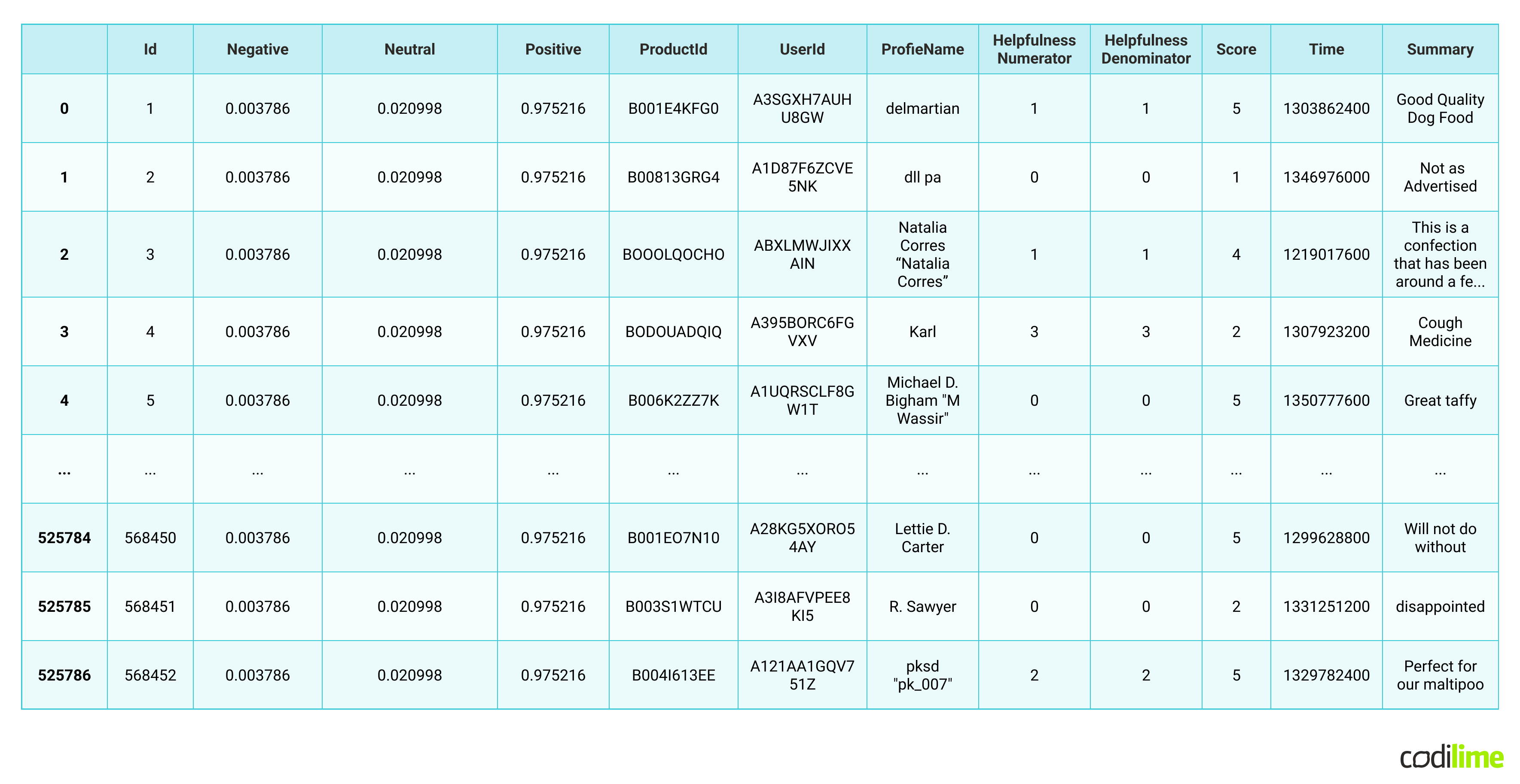
We can see now all the scores applied to each row - for each review. This is how RoBERTa could be used - without extra model training - just use an already existing model.

Is sentiment analysis accurate?

Data scientists still face many challenges while working with sentiment analysis models. For example, if a client wrote a review, “The product was white.” - referring to the fact that he received the wrong color item - this review would be classified with neutral sentiment because, considering the above - it does not bring any sentiment, whereas it should be classified as a negative sentiment. 

Another challenging situation for natural language processing would be using emojis. There is a whole different approach for a text which contains emojis, and we did not analyze it in this article, but you should also be aware and pay special attention to these kinds of models. 

On top of that, people can be contradictory in their reviews. Opinions could be very informal, and people are more likely to combine different points of view in the same statement, which makes it more challenging for a computer to understand. This means we still have a long way to go for accurate sentiment analysis. 

Check out our other articles about data engineering:

• What is data engineering?
• Top 20 data engineering software and tools
• SQL vs. NoSQL. The evolution of relational and non-relational databases

Moreover here, you can check our data science expertise in practice.

Conclusion

Sentiment analysis is a useful tool, but it is not a perfect one. Computers still have a long way to go to fully understand the nuances of human communication. However, using sentiment analysis can help in processing vast amounts of data much quicker than a human ever could. Natural language processing is a great tool to use to monitor the opinions and experiences of your customers.